SmarterEd

Aussie Maths & Science Teachers: Save your time with SmarterEd

  • Login
  • Get Help
  • About

Statistics, STD2 S1 2025 HSC 28

The heights of students in a class were recorded.

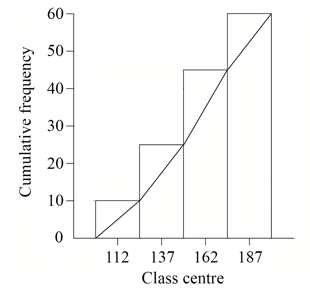
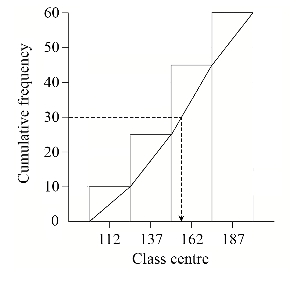
The results for this class are displayed in the cumulative frequency graph shown.


The shortest student in this class is 130 cm and the tallest student is 180 cm.

Construct a box-plot for this class in the space below.   (3 marks)
 

--- 7 WORK AREA LINES (style=lined) ---

Show Answers Only

Show Worked Solution

\(Q_1(7.5 \ \text{students })=135\)

\(Q_3(22.5 \ \text{students })=160\)

\(\text{Median (15 students )}=140\)
 

Filed Under: Bar Charts and Histograms (Std 2), Bar Charts and Histograms (Std2-2027), Summary Statistics - Box Plots (Std 2), Summary Statistics - Box Plots (Std2-2027) Tagged With: Band 5, smc-6310-30-Cumulative Frequency Histograms, smc-6313-30-Draw Box Plots, smc-821-20-Cumulative Frequency Histograms, smc-825-30-Draw Box-Plots

Statistics, STD2 S1 2022 HSC 15 MC

The cumulative frequency graph shows the distribution of the number of movie downloads made by 100 people in one month.
 

Which box-plot best represents the same data as displayed in the cumulative frequency graph?
 

Show Answers Only

`C`

Show Worked Solution

`text{1st quartile}\ ~~ 3`

`text{Median}\ ~~ 6`

`text{3rd quartile}\ ~~ 7`

`=>C`


♦♦♦ Mean mark 30%.

Filed Under: Bar Charts and Histograms (Std 2), Bar Charts and Histograms (Std2-2027), Summary Statistics - Box Plots (Std 2), Summary Statistics - Box Plots (Std2-2027) Tagged With: Band 6, common-content, smc-6310-30-Cumulative Frequency Histograms, smc-6310-40-IQR, smc-6313-10-Single Box Plots, smc-821-20-Cumulative Frequency Histograms, smc-821-30-IQR, smc-825-10-Single Box-Plots

Statistics, STD2 S1 2021 HSC 7 MC

The number of downloads of a song on each of twenty consecutive days is shown in the following graph.
 

Which of the following graphs best shows the cumulative number of downloads up to and including each day?

Show Answers Only

`C`

Show Worked Solution

`text{The gradient of the cumulative frequency histogram}`

♦ Mean mark 50%.

`text{will increase gradually, be steepest at day 10 then}`

`text{decrease gradually.}`

`=> C`

Filed Under: Bar Charts and Histograms (Std 2), Bar Charts and Histograms (Std2-2027) Tagged With: 2adv-std2-common, Band 5, common-content, smc-6310-30-Cumulative Frequency Histograms, smc-821-20-Cumulative Frequency Histograms

Statistics, STD2 S1 2020 HSC 7 MC

Which histogram best represents a dataset that is positively skewed?


Show Answers Only

`A`

Show Worked Solution

♦♦ Mean mark 32%.

`text(Positive skew occurs when the tail on the)`

`text{histogram is longer on the right-hand}`

`text{(positive) side.}`

`=> \ A`

Filed Under: Bar Charts and Histograms (Std 2), Bar Charts and Histograms (Std2-2027), Bar Charts and Histograms (Y12), Bar Charts, Histograms and Other Graphs (Std 1), Data Analysis Tagged With: Band 5, common-content, num-title-ct-core, num-title-qs-hsc, smc-1128-15-Histograms, smc-4224-35-Describing datasets, smc-6310-20-Histograms, smc-821-15-Histograms, smc-997-15-Histograms

Statistics, STD2 S1 2018 HSC 26d

The graph displays the mean monthly rainfall in Sydney and Perth.


  1. For how many months is the mean monthly rainfall higher in Perth than in Sydney?  (1 mark)

    --- 1 WORK AREA LINES (style=lined) ---

  2. For which of the two cities is the standard deviation of the mean monthly rainfall smaller? Justify your answer WITHOUT calculations.  (1 mark)

    --- 2 WORK AREA LINES (style=lined) ---

Show Answers Only
  1. `3`
  2. `text(The mean monthly rainfall of Sydney is in a)`
    `text(much tighter range than Perth.)`
    `:.\ text(Sydney has a smaller standard deviation.)`
Show Worked Solution

i.   `text(3 months (Jul, Aug and Sep))`

♦ Mean mark part (ii) 38%.
COMMENT: Extremely volatile result between parts with part (i) producing a 91% mean mark.


ii.    `text(The mean monthly rainfall of Sydney is in a)`

`text(much tighter range than Perth.)`

`:.\ text(Sydney has a smaller standard deviation.)`

Filed Under: Bar Charts and Histograms (Std 2), Bar Charts and Histograms (Std2-2027), Bar Charts and Histograms (Y12), Bar Charts, Histograms and Other Graphs (Std 1) Tagged With: Band 2, Band 5, common-content, smc-1128-10-Bar Charts, smc-6310-10-Bar Charts, smc-821-10-Bar Charts, smc-997-10-Bar Charts

Statistics, STD2 S1 2016 HSC 27c

The heights of 400 students were measured. The results are displayed in this cumulative frequency polygon.
 

2ug-2016-hsc-q27_2

 
Use the polygon to estimate the interquartile range.  (2 marks)

--- 4 WORK AREA LINES (style=lined) ---

Show Answers Only

`36\ text(cm)`

Show Worked Solution

`text(See graph for values:)`

♦ Mean mark 46%.

2ug-2016-hsc-q27c-answer

`IQR` `= Q_3 – Q_1`
  `= 172 – 136`
  `= 36\ text(cm)`

Filed Under: Bar Charts and Histograms, Bar Charts and Histograms (Std 2), Bar Charts and Histograms (Std2-2027), Bar Charts and Histograms (Y12), Bar Charts, Histograms and Other Graphs (Std 1) Tagged With: Band 5, common-content, smc-1128-20-Cumulative Frequency Histograms, smc-1128-30-IQR, smc-6310-30-Cumulative Frequency Histograms, smc-6310-40-IQR, smc-821-20-Cumulative Frequency Histograms, smc-821-30-IQR, smc-997-20-Cumulative Frequency Histograms, smc-997-30-IQR

Statistics, STD2 S1 2015 HSC 29d

Data from 200 recent house sales are grouped into class intervals and a cumulative frequency histogram is drawn.
 

2UG 2015 29d1 
 

  1. Use the graph to estimate the median house price.   (1 mark)

    --- 1 WORK AREA LINES (style=lined) ---

  2. By completing the table, calculate the mean house price.   (3 marks)

\begin{array} {|c|c|}
\hline
\rule{0pt}{2.5ex} \text{Class Centre} \rule[-1ex]{0pt}{0pt} & \text{Frequency} \\ \text{(\$'000)} &  \\
\hline
\rule{0pt}{2.5ex}  \rule[-1ex]{0pt}{0pt} &  \\
\hline
\rule{0pt}{2.5ex}  \rule[-1ex]{0pt}{0pt} &  \\
\hline
\rule{0pt}{2.5ex}  \rule[-1ex]{0pt}{0pt} &  \\
\hline
\rule{0pt}{2.5ex}  \rule[-1ex]{0pt}{0pt} & \\
\hline
\end{array}

--- 2 WORK AREA LINES (style=lined) ---

Show Answers Only
  1. `text(See Worked Solutions.)`
  2. `text(See Worked Solutions.)`
Show Worked Solution
i.   

2UG 2015 29d Answer

`text(From the graph, the estimated median)`

`text(house price = $392 500)`

♦♦♦ Mean marks of 9% for part (i) and 34% for part (ii)!

 
ii.

\begin{array} {|c|c|}
\hline
\rule{0pt}{2.5ex} \text{Class Centre} \rule[-1ex]{0pt}{0pt} & \text{Frequency} \\ \text{(\$’000)} &  \\
\hline
\rule{0pt}{2.5ex}  375 \rule[-1ex]{0pt}{0pt} & 30\\
\hline
\rule{0pt}{2.5ex}  385 \rule[-1ex]{0pt}{0pt} &  50 \\
\hline
\rule{0pt}{2.5ex}  395 \rule[-1ex]{0pt}{0pt} & 70 \\
\hline
\rule{0pt}{2.5ex}  405 \rule[-1ex]{0pt}{0pt} & 50 \\
\hline
\end{array}

 
`text(Mean house price ($’000))`

`= (375xx30 + 385xx50 + 395xx70 + 405xx50)/200`

`=$392`

`:. text(Mean house price is)\ $392\ 000`

Filed Under: Bar Charts and Histograms, Bar Charts and Histograms (Std 2), Bar Charts and Histograms (Std2-2027), Bar Charts and Histograms (Y12) Tagged With: Band 5, Band 6, common-content, smc-6310-30-Cumulative Frequency Histograms, smc-6310-50-Class Centres, smc-821-20-Cumulative Frequency Histograms, smc-821-40-Class Centres, smc-997-20-Cumulative Frequency Histograms, smc-997-40-Class Centres

Statistics, STD2 S1 2007 HSC 22 MC

A set of examination results is displayed in a cumulative frequency histogram and polygon (ogive).
 

2007 22 mc
 
Sanath knows that his examination mark is in the 4th decile.

Which of the following could have been Sanath’s examination mark?

  1.    37
  2.    57
  3.    67
  4.    77
Show Answers Only

`B`

Show Worked Solution

Data, 2UG 2007 HSC 22 MC Answer

`text(4th decile occurs when cumulative frequency)`

`text(is between 15 and 20.)`

`:.\ text(Examination mark must be between 55 and 60.)`

`=>  B`

Filed Under: Bar Charts and Histograms, Bar Charts and Histograms (Std 2), Bar Charts and Histograms (Std2-2027), Bar Charts and Histograms (Y12) Tagged With: Band 6, common-content, smc-6310-30-Cumulative Frequency Histograms, smc-821-20-Cumulative Frequency Histograms, smc-997-20-Cumulative Frequency Histograms

Statistics, STD2 S1 2006 HSC 24c

The heights of the 60 members of a choir were recorded. These results were grouped and then displayed as a cumulative frequency histogram and polygon.

The shortest person in the choir is 140 cm and the tallest is 190 cm.
 

2UG-2006-24c1

Draw an accurate box-and-whisker plot to represent the data.  (3 marks)

--- 8 WORK AREA LINES (style=lined) ---

Show Answers Only

`text{See Worked Solutions}`

Show Worked Solution

`text(Low) = 140`

`text(High) = 190`

`text(Median) = 150\ \ \ \ text{(# People = 30)}`

`Q_1 = 145\ \ \ \ text{(# People = 15)}`

`Q_3 = 170\ \ \ \ text{(# People = 45)}`

`text(Box and Whisker)`

HSC Data 13

Filed Under: Bar Charts and Histograms, Bar Charts and Histograms (Std 2), Bar Charts and Histograms (Std2-2027), Bar Charts and Histograms (Y12), Stem & Leaf, Box & Whisker, Summary Statistics - Box Plots (Std 2), Summary Statistics - Box Plots (Std2-2027), Summary Statistics - Box Plots (Y12) Tagged With: Band 5, common-content, smc-1000-30-Draw Box-Plots, smc-1128-20-Cumulative Frequency Histograms, smc-6310-30-Cumulative Frequency Histograms, smc-6313-30-Draw Box Plots, smc-821-20-Cumulative Frequency Histograms, smc-825-30-Draw Box-Plots, smc-997-20-Cumulative Frequency Histograms

Statistics, STD2 S1 2006 HSC 24a

2UG-2006-24a

List TWO ways in which this graph is misleading.  (2 marks)

--- 4 WORK AREA LINES (style=lined) ---

Show Answers Only

`text(Reasons the graph is misleading include)`

`text(- the columns are a different widths/volumes)`

`text(- the vertical axis doesn’t start at zero)`

Show Worked Solution

`text(Reasons the graph is misleading include)`

`text(- the columns are a different widths/volumes)`

`text(- the vertical axis doesn’t start at zero)`

Filed Under: Bar Charts and Histograms, Bar Charts and Histograms (Std 2), Bar Charts and Histograms (Std2-2027), Bar Charts and Histograms (Y12), Bar Charts, Histograms and Other Graphs (Std 1), Interpreting Data Tagged With: Band 4, common-content, num-title-ct-core, num-title-qs-hsc, smc-1128-10-Bar Charts, smc-5077-10-Misleading graphs, smc-6310-10-Bar Charts, smc-821-10-Bar Charts, smc-997-10-Bar Charts

Statistics, STD2 S1 2005 HSC 24d

The sector graph shows the proportion of people, as a percentage, living in each region of Sumcity. There are 24 000 people living in the Eastern Suburbs.
 

2UG-2005-24d1
 

  1. Show that the total number of people living in Sumcity is  160 000.  (1 mark)

    --- 1 WORK AREA LINES (style=lined) ---

Jake used the information above to draw a column graph.
 

2UG-2005-24d2

  1. The column graph height is incorrect for one region.


    Identify this region and justify your answer.   (2 marks)

    --- 4 WORK AREA LINES (style=lined) ---

Show Answers Only
  1. `160\ 000`
  2. `text(Western Suburbs population)`
Show Worked Solution

i.   `text(Let the population of Sumcity =)\ P`

`text(15%)× P` `= 24\ 000`
`:.P`  `= (24\ 000)/0.15` 
  `= 160\ 000\ …\ text(as required)` 


ii.  `text(Western Suburbs population)`

`= text(10%) × 160\ 000`

`= 16\ 000`

`text(The column graph has this population as)`

`text(12 000 people which is incorrect.)`

Filed Under: Bar Charts and Histograms, Bar Charts and Histograms (Std 2), Bar Charts and Histograms (Std2-2027), Bar Charts and Histograms (Y12), Bar Charts, Histograms and Other Graphs (Std 1), Displaying Data, Other Chart Types (Y12), Other Charts (Std 2), Other Charts (Std2-2027), Other Graphs Tagged With: Band 4, common-content, num-title-ct-core, num-title-qs-hsc, smc-1128-10-Bar Charts, smc-5076-15-Sector graphs and Divided Bar graphs, smc-5077-10-Misleading graphs, smc-6310-10-Bar Charts, smc-6311-30-Other Charts, smc-821-10-Bar Charts, smc-822-40-Other Charts, smc-997-10-Bar Charts, smc-998-40-Other Charts

Statistics, STD2 S1 2005 HSC 9 MC

A set of data is represented by the cumulative frequency histogram and ogive.
 

2UG-2005-9MC
 

What is the best approximation for the interquartile range for this set of data?

  1.    25
  2.    30
  3.    35
  4.    40
Show Answers Only

`C`

Show Worked Solution

2UG-2005-9MC Answer

`IQR` `= Q3 − Q1`
  `= 80 − 45`
  `= 35`

`=>  C`

Filed Under: Bar Charts and Histograms, Bar Charts and Histograms (Std 2), Bar Charts and Histograms (Std2-2027), Bar Charts and Histograms (Y12), Bar Charts, Histograms and Other Graphs (Std 1) Tagged With: Band 5, common-content, smc-1128-20-Cumulative Frequency Histograms, smc-1128-30-IQR, smc-6310-30-Cumulative Frequency Histograms, smc-6310-40-IQR, smc-821-20-Cumulative Frequency Histograms, smc-821-30-IQR, smc-997-20-Cumulative Frequency Histograms, smc-997-30-IQR

Statistics, STD2 S1 2008 HSC 26d

The graph shows the predicted population age distribution in Australia in 2008.


  1. How many females are in the 0–4 age group?  (1 mark)

    --- 1 WORK AREA LINES (style=lined) ---

  2. What is the modal age group?   (1 mark)

    --- 1 WORK AREA LINES (style=lined) ---

  3. How many people are in the 15–19 age group?   (2 marks)

    --- 4 WORK AREA LINES (style=lined) ---

  4. Give ONE reason why there are more people in the 80+ age group than in the 75–79 age group.   (1 mark)

    --- 2 WORK AREA LINES (style=lined) ---

Show Answers Only
  1. `600\ 000`
  2. `35-39`
  3. `1\ 450\ 000`
  4. `text(The 80+ group includes all people over 80)`
  5.  

    `text(and is not restricted by a 5-year limit.)`

Show Worked Solution
i.    `text{# Females (0-4)}` `= 0.6 xx 1\ 000\ 000`
    `= 600\ 000`


ii.    `text(Modal age group)\ =` `text(35 – 39)`


iii.   `text{# Males (15-19)}` `= 0.75 xx 1\ 000\ 000`
    `= 750\ 000`


`text{# Females (15-19)}` `= 0.7 xx 1\ 000\ 000`
  `= 700\ 000`


`:.\ text{Total People (15-19)}` `= 750\ 000 + 700\ 000`
  `= 1\ 450\ 000`


iv.   `text(The 80+ group includes all people over 80)`
  `text(and is not restricted by a 5-year limit.)`

Filed Under: Bar Charts and Histograms, Bar Charts and Histograms (Std 2), Bar Charts and Histograms (Std2-2027), Bar Charts and Histograms (Y12), Bar Charts, Histograms and Other Graphs (Std 1), Data Analysis Tagged With: Band 3, Band 4, Band 5, common-content, num-title-ct-core, num-title-qs-hsc, smc-1128-15-Histograms, smc-4224-15-Mode, smc-4224-35-Describing datasets, smc-6310-20-Histograms, smc-821-15-Histograms, smc-997-15-Histograms

Statistics, STD2 S1 2014 HSC 26e

The times taken for 160 music downloads were recorded, grouped into classes and then displayed using the cumulative frequency histogram shown.   


On the diagram, draw the lines that are needed to find the median download time.   (2 marks)

--- 0 WORK AREA LINES (style=lined) ---

Show Answers Only

Show Worked Solution
♦♦♦ Mean mark 17%.

HSC 2014 26ei

Filed Under: Bar Charts and Histograms, Bar Charts and Histograms (Std 2), Bar Charts and Histograms (Std2-2027), Bar Charts and Histograms (Y12) Tagged With: Band 6, common-content, smc-6310-30-Cumulative Frequency Histograms, smc-821-20-Cumulative Frequency Histograms, smc-997-20-Cumulative Frequency Histograms

Statistics, STD2 S1 2011 HSC 25b

The graph below displays data collected at a school on the number of students
in each Year group, who own a mobile phone.
 

2UG 2011 25b
 

  1. Which Year group has the highest percentage of students with mobile phones? (1 mark)

    --- 1 WORK AREA LINES (style=lined) ---

  2. Two students are chosen at random, one from Year 9 and one from Year 10.


    Which student is more likely to own a mobile phone?


    Justify your answer with suitable calculations. (2 marks)

    --- 4 WORK AREA LINES (style=lined) ---

  3. Identify a trend in the data shown in the graph. (1 mark)

    --- 2 WORK AREA LINES (style=lined) ---

Show Answers Only
  1. `text{Year 12 (100%)}`
  2. `text(Year 10)`
  3. `text(See Worked Solutions for detail)`
Show Worked Solution

i.   `text(Year 12 (100%))`

MARKER’S COMMENT: Many students ignore the instruction to use calculations and lose marks as a result.
 

ii.     `text(% Ownership in Year 9)` `=55/70`
    `=\ text{78.6%  (1d.p.)}`
      `text(% Ownership in Year 10)` `=50/60`
    `=\ text{83.3%  (1d.p.)}`

  
`:.\ text(The Year 10 student is more likely to own a mobile phone.)`


iii.   `text(% Ownership increases as students)`

 `text(progress from Year 7 to Year 12.)`

Filed Under: Bar Charts and Histograms, Bar Charts and Histograms (Std 2), Bar Charts and Histograms (Std2-2027), Bar Charts and Histograms (Y12), Bar Charts, Histograms and Other Graphs (Std 1), Displaying Data, Relative Frequency Tagged With: Band 3, Band 4, common-content, num-title-ct-core, num-title-qs-hsc, smc-1128-10-Bar Charts, smc-5076-10-Column graphs and histograms, smc-6310-10-Bar Charts, smc-821-10-Bar Charts, smc-997-10-Bar Charts

Statistics, STD2 S1 2010 HSC 26b

A new shopping centre has opened near a primary school. A survey is conducted to determine the number of motor vehicles that pass the school each afternoon between 2.30 pm and 4.00 pm.

The results for 60 days have been recorded in the table and are displayed in the cumulative frequency histogram.
 

2010 26b

  1. Find the value of  Χ  in the table.   (1 mark)

    --- 1 WORK AREA LINES (style=lined) ---

  2. On the cumulative frequency histogram above, draw a cumulative frequency polygon (ogive) for this data.   (1 mark)
  3. Use your graph to determine the median. Show, by drawing lines on your graph, how you arrived at your answer.   (1 mark)
  4. Prior to the opening of the new shopping centre, the median number of motor vehicles passing the school between  2.30 pm  and  4.00 pm  was 57 vehicles per day.


    What problem could arise from the change in the median number of motor vehicles passing the school before and after the opening of the new shopping centre?


    Briefly recommend a solution to this problem.   (2 marks)

    --- 5 WORK AREA LINES (style=lined) ---

Show Answers Only
  1. `15`
  2.  
  3.  
  4. `text(Problems)`
  5. `text(- increased traffic delays)`
  6. `text(- increased danger to students leaving school)`
  7.  

    `text(Solutions)`

  8. `text(- signpost alternative routes around school)`
  9. `text(- decrease the speed limit in the area)`
Show Worked Solution
i. `X` `= 25\ -10`
    `= 15`


♦♦♦ Mean mark 18%
MARKER’S COMMENT: The ogive was poorly drawn with many students incorrectly joining the middle of each column rather than from corner to corner.
ii.
♦♦ Mean mark 25%
MARKER’S COMMENT: Many students did not “show by drawing lines on the graph” as the question asked.

iii.  `text(Median)\ ~~155`

♦ Mean mark 47%
MARKER’S COMMENT: Short answers were often the best. Be concise when you can.
iv. `text(Problems)`
  `text(- increased traffic delays)`
  `text(- increased danger to students leaving school)`
   
  `text(Solutions)`
  `text(- signpost alternative routes around school)`
  `text(- decrease the speed limit in the area)`

Filed Under: Bar Charts and Histograms, Bar Charts and Histograms (Std 2), Bar Charts and Histograms (Std2-2027), Bar Charts and Histograms (Y12) Tagged With: Band 3, Band 5, Band 6, common-content, page-break-before-question, page-break-before-solution, smc-1128-40-Class Centres, smc-6310-30-Cumulative Frequency Histograms, smc-6310-50-Class Centres, smc-821-20-Cumulative Frequency Histograms, smc-821-40-Class Centres, smc-997-20-Cumulative Frequency Histograms, smc-997-40-Class Centres

Statistics, STD2 S1 2013 HSC 27c

A retailer has collected data on the number of televisions that he sold each week in 2012.

He grouped the data into classes and displayed the data using a cumulative frequency histogram and polygon (ogive).
 

2013 27c

  1. Use the cumulative frequency polygon to determine the interquartile range.  (2 marks)

    --- 4 WORK AREA LINES (style=lined) ---

  2. Oscar said that the retailer sold 300 televisions in 6 of the weeks in 2012.


    Is he correct? Give a reason for your answer.   (1 mark)

    --- 2 WORK AREA LINES (style=lined) ---

Show Answers Only
  1. `280`
  2. `text(Oscar is not correct because the data is grouped.)`
  3.  

    `text(He could only say that the retailer sold between 250`

  4.  

    `text(and 350 units in 6 of the weeks in 2012.)`

Show Worked Solution

i.  `text(S)text(ince cumulative frequency = 52 at max)`

♦♦♦ Mean mark 13%
COMMENT: Finding median and quartile values from cumulative frequency charts is an important skill that is often examined.

`=> text(Lower quartile at week) = 52/4 = 13`

`text(Lower quartile = 190)\ \ \ \ text{(from graph)}`

`=> text(Upper quartile at week) = 3 xx 13 = 39`

`text(Upper quartile = 470)`

`:.\ text(IQR)`  `= 470` `-190`
  `=280`


ii.  `text(Oscar is not correct because the data is grouped.)`

♦♦♦ This question proved a beast, with a mean mark of 1%. Toughest question in the 2013 exam!

`text(He could only say the retailer sold between)`

`text(250 and 350 units in 6 of the weeks in 2012.)`

Filed Under: Bar Charts and Histograms, Bar Charts and Histograms (Std 2), Bar Charts and Histograms (Std2-2027), Bar Charts and Histograms (Y12) Tagged With: Band 6, common-content, smc-6310-30-Cumulative Frequency Histograms, smc-6310-40-IQR, smc-821-20-Cumulative Frequency Histograms, smc-821-30-IQR, smc-997-20-Cumulative Frequency Histograms, smc-997-30-IQR

Probability, STD2 S2 2010 HSC 23c

On Saturday, Jonty recorded the colour of T-shirts worn by the people at his gym. The results are shown in the graph.


  1. How many people were at the gym on Saturday? (Assume everyone was wearing a T-shirt).   (1 mark)

    --- 1 WORK AREA LINES (style=lined) ---

  2. What is the probability that a person selected at random at the gym on Saturday, would be wearing either a blue or green T-shirt?   (1 mark)

    --- 2 WORK AREA LINES (style=lined) ---

Show Answers Only
  1. `34`
  2. `15/34`
Show Worked Solution
i.   `text(# People)` `=5+15+10+3+1`
  `=34`


ii.   `P (B\ text{or}\ G)` `=P(B)+P(G)`
  `=5/34+10/34`
  `=15/34`

Filed Under: Bar Charts and Histograms, Bar Charts and Histograms (Std 2), Bar Charts and Histograms (Std2-2027), Bar Charts and Histograms (Y12), Combinations and Single Stage Events (Std 2), Probability, Single and Multi-Stage Events (Std 1), Single stage events Tagged With: Band 2, Band 3, common-content, num-title-ct-core, num-title-qs-hsc, smc-1135-05-Simple Probability, smc-4225-15-Single-stage events, smc-6310-10-Bar Charts, smc-821-10-Bar Charts, smc-828-10-Simple Probability, smc-997-10-Bar Charts

Statistics, STD2 S1 2011 HSC 11 MC

The sets of data, `X` and `Y`, are displayed in the histograms.

2UG 2011 11

Which of these statements is true?

  1.   `X` has a larger mode and `Y ` has a larger range.
  2.   `X` has a larger mode and the ranges are the same.
  3.   The modes are the same and `Y` has a larger range.
  4.   The modes are the same and the ranges are the same.
Show Answers Only

`B`

Show Worked Solution
♦ Mean mark 47%

`text(Mode of)\ X=9`

`text(Range of)\ X=9-3=6`

`text(Mode of)\ Y=8`

`text(Range of)\ Y=11-5=6`

`:. X\ text(has a larger mode and ranges are the same)`

`=>B`

Filed Under: Bar Charts and Histograms, Bar Charts and Histograms (Std 2), Bar Charts and Histograms (Std2-2027), Bar Charts and Histograms (Y12), Bar Charts, Histograms and Other Graphs (Std 1), Data Analysis Tagged With: Band 4, common-content, num-title-ct-core, num-title-qs-hsc, smc-1128-15-Histograms, smc-4224-45-Mean/median/mode/range, smc-6310-20-Histograms, smc-821-15-Histograms, smc-997-15-Histograms

Statistics, STD2 S5 2010 HSC 4 MC

Which of the following frequency histograms shows data that could be normally distributed?
 

Capture1

Capture2 

Show Answers Only

`A`

Show Worked Solution

`text(Normally distributed data have a frequency)`

`text(histogram graph that is shaped like a bell.)`

`=>  A`

Filed Under: Bar Charts and Histograms, Bar Charts and Histograms (Std 2), Bar Charts and Histograms (Std2-2027), Bar Charts and Histograms (Y12), DS5/6 - Normal Distribution and Sampling, Normal Distribution (Y12), S5 The Normal Distribution (Y12) Tagged With: Band 4, common-content, smc-6310-20-Histograms, smc-819-40-Graphs, smc-821-15-Histograms, smc-995-40-Graphs, smc-997-15-Histograms

Statistics, STD2 S1 2013 HSC 15 MC

The frequency histogram shows the number of goals scored by a football team in each game in a season.
 

2013 15 mc

 
What is the mean number of goals scored per game by this team?

  1.    4
  2.    4.5
  3.    5
  4.    5.5
Show Answers Only

`C`

Show Worked Solution

`text(Total number of goals scored)`

`=(3xx3)+(4xx7)+(5xx5)+(6xx1)+(7xx0)+(8xx4)`

`=9+28+25+6+0+32`

`=100`

`text(Number of games)=3+7+5+1+4=20`

`:.\ text(Mean goals per game)=100/20=5`

`=>\ C`

Filed Under: Bar Charts and Histograms, Bar Charts and Histograms (Std 2), Bar Charts and Histograms (Std2-2027), Bar Charts and Histograms (Y12), Bar Charts, Histograms and Other Graphs (Std 1), Data Analysis Tagged With: Band 4, common-content, num-title-ct-core, num-title-qs-hsc, smc-1128-15-Histograms, smc-4224-25-Mean, smc-6310-20-Histograms, smc-821-15-Histograms, smc-997-15-Histograms

Statistics, STD2 S1 2013 HSC 6 MC

A survey was conducted where people were asked which of two brands of smartphones they preferred. The results were:

  • 48% preferred Brand X
  • 52% preferred Brand Y

A graph displaying the data is to be included in a magazine article. The editor of the magazine wishes to ensure that the graph is not misleading in any way.

Which graph should the editor choose to include in the article?
 

2013 6 mc1

2013 6 mc2

Show Answers Only

`D`

Show Worked Solution

`D\ text(is the best as it starts at zero on the)\ y text(-axis)`

`text(and has the same column widths.)`

Filed Under: Bar Charts and Histograms, Bar Charts and Histograms (Std 2), Bar Charts and Histograms (Std2-2027), Bar Charts and Histograms (Y12), Bar Charts, Histograms and Other Graphs (Std 1), Interpreting Data Tagged With: Band 4, common-content, num-title-ct-core, num-title-qs-hsc, smc-1128-10-Bar Charts, smc-6310-10-Bar Charts, smc-821-10-Bar Charts, smc-997-10-Bar Charts

Copyright © 2014–2025 SmarterEd.com.au · Log in