If `f(x)=log_2(x^(2x))`, which expression is equal to `f^(′)(x)`?
- `2/(x^(2x)ln2`
- `2/ln2 + 2log_2x`
- `log_2x+2/ln2`
- `2/ln2 xx log_2(x^(2x-1))`
Aussie Maths & Science Teachers: Save your time with SmarterEd
If `f(x)=log_2(x^(2x))`, which expression is equal to `f^(′)(x)`?
The zoo’s management requests quotes for parts of the new building works.
Four businesses each submit quotes for four different tasks.
Each business will be offered only one task.
The quoted cost, in $100 000, of providing the work is shown in Table 1 below.

The zoo’s management wants to complete the new building works at minimum cost.
The Hungarian algorithm is used to determine the allocation of tasks to businesses.
The first step of the Hungarian algorithm involves row reduction; that is, subtracting the smallest element in each row of Table 1 from each of the elements in that row.
The result of the first step is shown in Table 2 below.

The second step of the Hungarian algorithm involves column reduction; that is, subtracting the smallest element in each column of Table 2 from each of the elements in that column.
The results of the second step of the Hungarian algorithm are shown in Table 3 below. The values of Task 1 are given as `A, B, C` and `D`.

--- 1 WORK AREA LINES (style=lined) ---
Draw these three lines on Table 3 above. (1 mark)
--- 0 WORK AREA LINES (style=lined) ---
When all steps of the Hungarian algorithm are complete, a bipartite graph can show the allocation for minimum cost.
Complete the bipartite graph below to show this allocation for minimum cost. (1 mark)
--- 4 WORK AREA LINES (style=lined) ---

How much is this reduction? (1 mark)
--- 6 WORK AREA LINES (style=lined) ---
a. `A = 2, \ B = 1, \ C = 1, \ D = 0`
| b. |  |
c. `text(After next step:)`

`text(Allocation): `

d. `text{Hungarian Algorithm table (complete):}`

`text(Allocation): B2 -> T3,\ B1 -> T4,\ B3 -> T2,\ B4 -> T1`
`text(C)text(ost) = 4 + 7 + 8 + 10 = 29`
`text(Previous cost) = 5 + 10 + 8 + 8 = 31`
| `:.\ text(Reduction)` | `= 2 xx 100\ 000` |
| `= $200\ 000` |
A cake in the shape of three cylindrical sections is shown in the diagram below.

Each section of the cake has a height of 8 cm, as shown in the diagram.
The middle section of the cake, B, has twice the volume of the top section of the cake, A.
The bottom section of the cake, C, has twice the volume of the middle section of the cake, B.
The volume of the top section of the cake, A, is 900 cm3.
The diameter of the bottom section of the cake, C, in centimetres, is closest to
The cities of Lima and Washington, DC have the same longitude of 77° W.
The shortest great circle distance between Lima and Washington, DC is 5697 km.
Assume that the radius of Earth is 6400 km.
Lima has a latitude of 12° S and is located due south of Washington, DC.
What is the latitude of Washington, DC?

| `text(Arc Distance) \ WL` | `= 5697` |
| `({theta + 12}/{360}) xx 2 xx pi xx 6400` | `= 5697` |
| `theta + 12` | `= (5697 xx 360)/(2 pi xx 6400)` |
| `= 51°` | |
| `:. \ theta` | `= 39°` |
`=> \ A`
A waterfall in a national park is 4 km east of a camp site.
A lookout tower is 4 km south of the waterfall.
The bearing of the camp site from the lookout tower is

| `text(Bearing of) \ C \ text(from) \ T` | `= 360 – 45` |
| `= 315°` |
`=> \ E`
The construction of the new reptile exhibit is a project involving nine activities, `A` to `I`.
The directed network below shows these activities and their completion times in weeks.

--- 1 WORK AREA LINES (style=lined) ---
--- 1 WORK AREA LINES (style=lined) ---
--- 2 WORK AREA LINES (style=lined) ---
a. `D, G and I`
b. `text(Scanning forwards and backwards:)`

`text(Critical Path:)\ ACDFGI`
| c. | `text{LST (activity}\ B text{)}` | `= 7 – 5` |
| `= 2\ text(weeks)` |
A zoo has an entrance, a cafe and nine animal exhibits: bears `(B)`, elephants `(E)`, giraffes `(G)`, lions `(L)`, monkeys `(M)`, penguins `(P)`, seals `(S)`, tigers `(T)` and zebras `(Z)`.
The edges on the graph below represent the paths between the entrance, the cafe and the animal exhibits. The numbers on each edge represent the length, in metres, along that path. Visitors to the zoo can use only these paths to travel around the zoo.

--- 1 WORK AREA LINES (style=lined) ---
--- 1 WORK AREA LINES (style=lined) ---
--- 0 WORK AREA LINES (style=lined) ---

A reptile exhibit `(R)` will be added to the zoo.
A new path of length 20 m will be built between the reptile exhibit `(R)` and the giraffe exhibit `(G)`.
A second new path, of length 35 m, will be built between the reptile exhibit `(R)` and the cafe.
--- 0 WORK AREA LINES (style=lined) ---
By how many metres will these new paths reduce the minimum distance between the giraffe exhibit `(G)` and the cafe? (1 mark)
--- 5 WORK AREA LINES (style=lined) ---
a. `45\ text(metres)`
b.i. `text(Hamilton cycle.)`
| b.ii. |  |
`text(Possible route:)`
`text(entrance)\ – LGTMCEBSZP\ –\ text(entrance)`
| c. |  |
d. `text{Minimum distance (before new exhibit)}`
`= GLTMC`
`= 15 + 35 + 40 + 50`
`= 140\ text(m)`
`:.\ text(Reduction in minimum distance)`
`= 140 – (20 + 35)`
`= 85\ text(m)`
After 5.00 pm, tourists will start to arrive in Gillen and they will stay overnight.
As a result, the number of people in Gillen will increase and the television viewing habits of the tourists will also be monitored.
Assume that 50 tourists arrive every hour.
It is expected that 80% of arriving tourists will watch only `C_2` during the hour that they arrive.
The remaining 20% of arriving tourists will not watch television during the hour that they arrive.
Let `W_m` be the state matrix that shows the number of people in each category `m` hours after 5.00 pm on this day.
The recurrence relation that models the change in the television viewing habits of this increasing number of people in Gillen `m` hours after 5.00 pm on this day is shown below.
`W_(m + 1) = TW_m + V`
where
`{:(quad qquad qquad qquadqquadqquadquadtext(this hour)),(qquadqquadqquad quad \ C_1 qquad quad C_2 qquad \ C_3 quad \ NoTV),(T = [(quad 0.50, 0.05, 0.10, 0.20 quad),(quad 0.10, 0.60, 0.20, 0.20 quad),(quad 0.25, 0.10, 0.50, 0.10 quad),(quad 0.15, 0.25, 0.20, 0.50 quad)]{:(C_1),(C_2),(C_3),(NoTV):}\ text(next hour,) qquad and qquad W_0 = [(400), (600), (300),(700)]):}`
--- 3 WORK AREA LINES (style=lined) ---
--- 5 WORK AREA LINES (style=lined) ---
The basketball finals will be televised on `C_3` from 12.00 noon until 4.00 pm.
It is expected that 600 Gillen residents will be watching `C_3` at any time from 12.00 noon until 4.00 pm.
The remaining 1400 Gillen residents will not be watching `C_3` from 12.00 noon until 4.00 pm (represented by NotC3).
`{:(qquadqquadqquadquadtext(this hour)),(qquadqquadqquad \ C_3 quadquad \ NotC_3),(P = [(v, qquad quad w quad),(0.35, quad qquad x quad)]{:(C_3),(NotC_3):}\ text(next hour)):}`
Write down the values of `v, w` and `x` in the boxes provided below. (2 marks)
| `v =` |
|
`w =` |
|
`x =` |
|
--- 6 WORK AREA LINES (style=lined) ---
Three television channels, `C_1, C_2` and `C_3`, will broadcast the International Games in Gillen.
Gillen’s 2000 residents are expected to change television channels from hour to hour as shown in the transition matrix `T` below.
The option for residents not to watch television (NoTV) at that time is also indicated in the transition matrix.
`{:(qquadqquadqquadqquadqquadquadtext(this hour)),(qquadqquadqquad \ C_1 quadquad \ C_2 quadqquad C_3 quad \ NoTV),(T = [(0.50,0.05,0.10,0.20),(0.10,0.60,0.20,0.20),(0.25,0.10,0.50,0.10),(0.15,0.25,0.20,0.50)]{:(C_1),(C_2),(C_3),(NoTV):}text(next hour)):}`
The state matrix `G_0` below lists the number of Gillen residents who are expected to watch the games on each of the channels at the start of a particular day (9.00 am).
Also shown is the number of Gillen residents who are not expected to watch television at that time.
`G_0 = [(100), (400), (100), (1400)]{:(C_1), (C_2), (C_3), (NoTV):}`
--- 0 WORK AREA LINES (style=lined) ---
|
|
`xx 100 +` |
|
`xx 400 +` |
|
`xx 100 ` |
| `+\ \ ` |
|
`xx 1400 ` | `= 835` |
--- 3 WORK AREA LINES (style=lined) ---
A total of six residents from two towns will be competing at the International Games.
Matrix `A`, shown below, contains the number of male `(M)` and the number of female `(F)` athletes competing from the towns of Gillen `(G)` and Haldaw `(H)`.
`{:(qquad qquad quad \ M quad F), (A = [(2, 2), (1, 1)]{:(G),(H):}):}`
--- 1 WORK AREA LINES (style=lined) ---
Each of the six athletes will compete in one event: table tennis, running or basketball.
Matrices `T` and `R`, shown below, contain the number of male and female athletes from each town who will compete in table tennis and running respectively.
| Table tennis | Running | |
|
`{:(qquad qquad quad \ M quad F), (T = [(0, 1), (1, 0)]{:(G),(H):}):}` |
`{:(qquad qquad quad \ M quad F), (R = [(1, 1), (0, 0)]{:(G),(H):}):}` |
Complete matrix `B` below. (1 mark)
--- 0 WORK AREA LINES (style=lined) ---
`{:(qquad qquad qquad \ M qquad quad F), (B = [(\ text{___}, text{___}\ ), (\ text{___}, text{___}\)]{:(G),(H):}):}`
Matrix `C` contains the cost of one uniform, in dollars, for each of the three events: table tennis `(T)`, running `(R)` and basketball `(B)`.
`C = [(515), (550), (580)]{:(T), (R), (B):}`
--- 1 WORK AREA LINES (style=lined) ---
--- 3 WORK AREA LINES (style=lined) ---
--- 0 WORK AREA LINES (style=lined) ---
`Q = [(1, text{___}, text{___}\ ), (0, 0, 1), (0, 1, 1), (\ text{___}, text{___}, 0)]`
Evaluate `int_0^1 e^x - e^-x\ dx`. (2 marks)
Let `f(x) = -x^2 + x + 4` and `g(x) = x^2 - 2`.
--- 6 WORK AREA LINES (style=lined) ---
--- 4 WORK AREA LINES (style=lined) ---
Let `overset^p` be the random variable that represents the sample proportions of customers who bring their own shopping bags to a large shopping centre. From a sample consisting of all customers on a particular day, an approximate 95% confidence interval for the proportion `p` of customers who bring their own shopping bags to this large shopping centre was determined to be `((4853)/(50\ 000) , (5147)/(50\ 000))`. --- 3 WORK AREA LINES (style=lined) --- --- 5 WORK AREA LINES (style=lined) ---
Let `f : [ 0, (pi)/(2)] → R, \ f(x) = 4 cos(x)` and `g : [0, (pi)/(2)] → R, \ g(x) = 3 sin(x)`.
--- 0 WORK AREA LINES (style=lined) ---
`qquad qquad `
Find the value of `sin(c)` and the value of `cos(c)`. (3 marks)
--- 4 WORK AREA LINES (style=lined) ---
--- 0 WORK AREA LINES (style=lined) ---
--- 7 WORK AREA LINES (style=lined) ---
a.

b. `text(At intersection:)`
| `4cos(c)` | `= 3sin(c)` |
| `tan(c)` | `= (4)/(3)` |

`sin(c) = (4)/(5)`
`cos(c) = (3)/(5)`
c. i.

| ii. `A` | `= int_0^c g(x)\ dx + int_c^((pi)/(2)) f(x)\ dx` |
| `= int_0^c 3sin x \ dx + int_c^((pi)/(2)) 4cos \ x \ dx` | |
| `= 3[-cos x]_0^c + 4[sin x]_c^((pi)/(2))` | |
| `= 3(-cos(c) + cos \ 0) + 4(sin \ (pi)/(2)-sin(c))` | |
| `= 3(-(3)/(5) + 1) + 4(1-(4)/(5))` | |
| `= (6)/(5) + (4)/(5)` | |
| `= 2 \ \ text(u²)` |
The discrete random variable `X` has the probability mass function `text(Pr)(X = x) = {(kx), (k), (0):} qquad {:(x∈{1, 4, 6}), (x = 3), (text(otherwise)):}` --- 5 WORK AREA LINES (style=lined) --- --- 5 WORK AREA LINES (style=lined) --- --- 5 WORK AREA LINES (style=lined) ---
Solve `log_3(t) - log_3(t^2 - 4) = -1` for `t`. (3 marks)
Evaluate `int_0^1 e^x-e^-x\ dx`. (2 marks)
--- 4 WORK AREA LINES (style=lined) ---
Let `f(x) = -x^2 + x + 4` and `g(x) = x^2-2`.
--- 4 WORK AREA LINES (style=lined) ---
Marty has been depreciating the value of his car each year using flat rate depreciation.
After three years of ownership, the value of the car was halved due to an accident.
Marty continued to depreciate the value of his car by the same amount each year after the accident.
Which one of the following graphs could show the value of Marty’s car after `n` years, `C_n`?
| A. |  |
B. |  |
| C. |  |
D. |  |
| E. |  |
Point `C` lies on `AB` such that `overset(->)(AC) = lambdaoverset(->)(AB)`.
--- 8 WORK AREA LINES (style=lined) ---
--- 4 WORK AREA LINES (style=lined) ---
| i. |  |
`underset~c = underset~a + overset(->)(AC)`
| `overset(->)(AB)` | `= underset~b-underset~a` |
| `overset(->)(AC)` | `= lambdaoverset(->)(AB)` |
| `= lamda(underset~b-underset~a)` |
| `:.underset~c` | `= underset~a + lambda(underset~b-underset~a)` |
| `= lambdaunderset~b + (1-lambda)underset~a` |
| ii. | `overset(->)(BC)` | `= underset~c-underset~b` |
| `= lambdaunderset~b + (1-lambda)underset~a-underset~b` | ||
| `=(1-lambda)underset~a +(lambda-1)underset~b` | ||
| `=(1-lambda)underset~a -(1-lambda)underset~b` | ||
| `= (1-lambda)(underset~a-underset~b)` |
Using vectors, calculate the acute angle between the line that passes through `A(1, 3)` and `B(2,–6)` and the line that passes through `C(1, 5)` and `D(3,–2)`.
Give your answer correct to one decimal place. (2 marks)
--- 6 WORK AREA LINES (style=lined) ---
A force described by the vector `underset~F = ((3),(6))` newtons is applied to a line `l` which is parallel to the vector `((4),(3))`.
--- 5 WORK AREA LINES (style=lined) ---
--- 2 WORK AREA LINES (style=lined) ---
In the diagram below, `ROT` is a diameter of the circle with centre `O`.
`S` is a point on the circumference.

Using the properties of vectors `underset~r`, `underset~s` and `underset~t`, show that `angleRST` is a right angle. (2 marks)
--- 8 WORK AREA LINES (style=lined) ---
Tisha plays drums in the same band as Marlon.
She would like to buy a new drum kit and has saved $2500.
The balance of this investment after `n` months, `T_n` could be determined using the recurrence relation below
`T_0 = 2500, \ \ \ \ T_(n+1) = 1.0036 xx T_n`
Calculate the total interest that would be earned by Tisha's investment in the first five months.
Round your answer to the nearest cent. (2 marks)
--- 4 WORK AREA LINES (style=lined) ---
Tisha could invest the $2500 in a different account that pays interest at the rate of 4.08% per annum, compounding monthly. She would make a payment of $150 into this account every month.
Write down a recurrence relation, in terms of `V_0`, `V_n` and `V_(n + 1)`, that would model the change in the value of this investment. (1 mark)
--- 2 WORK AREA LINES (style=lined) ---
What annual interest rate would Tisha require?
Round your answer to two decimal places. (1 mark)
--- 2 WORK AREA LINES (style=lined) ---
Marlon plays guitar in a band.
He paid $3264 for a new guitar.
The value of Marlon's guitar will be depreciated by a fixed amount for each concert that he plays.
After 25 concerts, the value of the guitar will have decreased by $200.
--- 2 WORK AREA LINES (style=lined) ---
--- 2 WORK AREA LINES (style=lined) ---
Complete the rule below by writing the appropriate numbers in the boxes provided. (1 mark)
--- 1 WORK AREA LINES (style=lined) ---
`G_n =` – × `n`
After how many concerts will the value of Marlon's guitar first fall below $2500? (2 marks)
--- 4 WORK AREA LINES (style=lined) ---
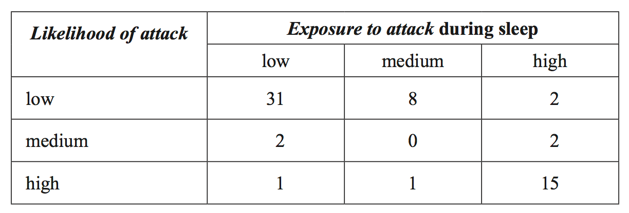
A random sample of 12 mammals drawn from a population of 62 types of mammals was categorized according to two variables. likelihood of attack (1 = low, 2 = medium, 3 = high) exposure to attack during sleep (1 = low, 2 = medium, 3 = high) The data is shown in the following table. --- 0 WORK AREA LINES (style=lined) --- The following two-way frequency table was formed from the data generated when the entire population of 62 types of mammals was similarly categorized. --- 5 WORK AREA LINES (style=lined) --- --- 2 WORK AREA LINES (style=lined) --- --- 4 WORK AREA LINES (style=lined) ---


Show Answers Only

`= 50 %`
`text(of attack is associated with low exposure to attack during sleep.)`
`text(- 91%) \ ({31}/{34}) \ text(of animals with low exposure to attack)`
`text(during sleep, have a low likelihood of attack.)`
`text(- Similarly, 89% of animals with a medium exposure to attack during)`
`text(sleep have a low likelihood of attack.)`
`text(- 11% of animals with a high exposure to attack during sleep have)`
`text(a low likelihood of attack)`
a. b. i. `15` iii. `text(The data supports the contention that animals with a low likelihood)` `text(of attack is associated with low exposure to attack during sleep.)` `text(- 91%) \ ({31}/{34}) \ text(of animals with low exposure to attack)` `text(during sleep, have a low likelihood of attack.)` `text(- Similarly, 89% of animals with a medium exposure to attack during)` `text(sleep have a low likelihood of attack.)` `text(- 11% of animals with a high exposure to attack during sleep have)` `text(a low likelihood of attack)`Show Worked Solution
ii. `text(Percentage)`
`= (2)/(4) xx 100`
`= 50%`
The scatterplot below plots the variable life span, in years, against the variable sleep time, in hours, for a sample of 19 types of mammals.

On the assumption that the association between sleep time and life span is linear, a least squares line is fitted to this data with sleep time as the explanatory variable.
The equation of this least squares line is
life span = 42.1 – 1.90 × sleep time
The coefficient of determination is 0.416
--- 0 WORK AREA LINES (style=lined) ---
--- 2 WORK AREA LINES (style=lined) ---
--- 2 WORK AREA LINES (style=lined) ---
--- 2 WORK AREA LINES (style=lined) ---
--- 4 WORK AREA LINES (style=lined) ---

`text(Direction is negative.)`
`text(1.9 years for each additional hour of sleep time.)`
`text(variation in sleep time.)`
a. `text{Graph endpoints (0, 42.1) and (18, 7.9)}`
b. `text(Strength is moderate.)`
`text(Direction is negative.)`
c. `text(The gradient of –1.9 means that life span decreases by)`
`text(1.9 years for each additional hour of sleep time.)`
d. `text(41.6% of the variation in life span can be explained by the )`
`text(variation in sleep time.)`
| e. `text(Predicted value)` | `= 42.1 – 1.9 xx 12` |
| `= 19.3 \ text(years)` |
| `text(Residual)` | `= text(actual) – text(predicted)` |
| `= 39.2 – 19.3` | |
| `= 19.9 \ text(years)` |
The life span, in years, and gestation period, in days, for 19 types of mammals are displayed in the table below.

--- 1 WORK AREA LINES (style=lined) ---
--- 2 WORK AREA LINES (style=lined) ---
--- 2 WORK AREA LINES (style=lined) ---
The five-number summary below was determined from the sleep time, in hours, of a sample of 59 types of mammals. \begin{array} {|l|c|} --- 5 WORK AREA LINES (style=lined) --- --- 0 WORK AREA LINES (style=lined) ---
\hline
\rule{0pt}{2.5ex} \ \ \ \textbf{Statistic} \rule[-1ex]{0pt}{0pt} & \textbf{Sleep time (hours)} \\
\hline
\rule{0pt}{2.5ex} \text{minimum} \rule[-1ex]{0pt}{0pt} & \text{2.5} \\
\hline
\rule{0pt}{2.5ex} \text{first quartile} \rule[-1ex]{0pt}{0pt} & \text{8.0} \\
\hline
\rule{0pt}{2.5ex} \text{median} \rule[-1ex]{0pt}{0pt} & \text{10.5} \\
\hline
\rule{0pt}{2.5ex} \text{third quartile} \rule[-1ex]{0pt}{0pt} & \text{13.5} \\
\hline
\rule{0pt}{2.5ex} \text{maximum} \rule[-1ex]{0pt}{0pt} & \text{20.0} \\
\hline
\end{array}

Show Answers Only

a. `IQR = Q_3-Q_1 = 13.5-8.0 = 5.5` `=> \ text(no outliers)` b. Show Worked Solution
`text(Lower fence)`
`= Q_1-1.5 xx IQR`
`= 8-1.5 xx 5.5`
`= -0.25`
`text(Upper fence)`
`= Q_3 + 1.5 xx IQR`
`= 13.5 + 1.5 xx 5.5`
`= 21.75`
`text(S) text(ince) \ -0.25 < 2.5 \ text{(minimum value) and} \ 21.75 > 20.0 \ text{(maximum value)}`
The table below displays the average sleep time, in hours, for a sample of 19 types of mammals.

--- 1 WORK AREA LINES (style=lined) ---
--- 2 WORK AREA LINES (style=lined) ---
--- 2 WORK AREA LINES (style=lined) ---
--- 2 WORK AREA LINES (style=lined) ---
Four cards are placed face down on a table. The cards are made up of a Jack, Queen, King and Ace.
A gambler bets that she will choose the Queen in a random pick of one of the cards.
If this process is repeated 7 times, express the gambler's success as a Bernoulli random variable and calculate
--- 1 WORK AREA LINES (style=lined) ---
--- 1 WORK AREA LINES (style=lined) ---
In January 2018, an online shop had 260 customer accounts.
In June 2018, the shop had 500 customer accounts.
The graph below shows the number of customer accounts, `a`, with the online shop `n` months after January 2018, for a period of 10 months.

The growth in the number of customer accounts that this graph shows is expected to continue beyond these 10 months, following the same trend.
How many customer accounts can the online shop expect to have at the end of December 2019 `(n = 23)`?
The revenue, `R`, in dollars, that a company receives from selling `n` caps is given by the equation
`R = {(25n, qquad n <= 1000),(20n + c, qquad n> 1000):}`
The graph of this revenue equation consists of two straight lines that intersect at the point where `n = 1000`.
What is the value of `c` in this revenue equation?
The graph below shows a relationship between `x` and `y`.

The rule that represents this relationship between `x` and `y` is
Matrix `W` is a `3 xx 2` matrix.
Matrix `Q` is a matrix such that `Q xx W = W`.
Matrix `Q` could be
| A. | `\ [1]` | B. | `\ [(1,0),(0,1)]` | C. | `\ [(1,1),(1,1),(1,1)]` |
| D. | `\ [(1,0,0),(0,1,0),(0,0,1)]` | E. | `\ [(1,1,1),(1,1,1),(1,1,1)]` |
In a game between two teams, Hillside and Rovers, each team can score points in two ways.
The team may hit a Full or the team may hit a Bit.
More points are scored for hitting a Full than for hitting a Bit.
A team’s total point score is the sum of the points scored from hitting Fulls and Bits.
The table below shows the scores at the end of the game.

Let `f` be the number of points scored by hitting one Full.
Let `b` be the number of points scored by hitting one Bit.
Which one of the following matrix products can be evaluated to find the matrix `[(f),(b)]`?
| A. | `\ [(4,8),(5,2)]^(−1) xx [(52),(49)]` | B. | `\ [(4,8),(5,2)] xx [(52),(49)]` | C. | `\ [(52,49)][(4,8),(5,2)]` |
| D. | `\ [(52,49)][(4,8),(5,2)]^(−1)` | E. | `\ [(4,8,52),(5,2,49)]^(−1)` |
Four teams, blue (`B`), green (`G`), orange (`O`) and pink (`P`), played each other once in a competition.
There were no draws in this competition.
The results of the competition are shown in the matrix below.
`{:(),(),(text(winner)):}{:(qquadqquad\ text(loser)),((qquadquadB,G,O,P)),({: (B), (G), (O), (P):}[(text(−),1,v,1),(0,text(−),1,1),(0,w,text(−),0),(0,0,x,text(−))]):}`
The letters `v`, `w` and `x` each have a value of 0 or 1.
A 1 in the matrix shows that the team named in that row defeated the team named in that column.
A 0 in the matrix shows that the team named in that row was defeated by the team named in that column.
A dash (–) in the matrix shows that no game was played.
The values of `v`, `w` and `x` are
In the graph below, the vertices represent electricity transformer substations.
The numbers on the edges of the graph show the length, in kilometres, of cables that connect these substations.

What is the minimum length of cable, in kilometres, that is necessary to make sure that each substation remains connected to the network?

| `text(Minimum length)` | `= 7 + 8 + 10 + 7 + 9 + 8 + 11 + 11` |
| `= 71\ text(km)` |
`=> B`
Which one of the following flow diagrams shows a cut that has a capacity of 19?
| A. |  |
| B. |  |
| C. |  |
| D. |  |
| E. |  |
Let `f: R → R, \ f(x) = e^((x/2))` and `g: R → R, \ g(x) = 2log_e(x)`.
--- 4 WORK AREA LINES (style=lined) ---
--- 5 WORK AREA LINES (style=lined) ---
--- 3 WORK AREA LINES (style=lined) ---
Let `B` be the point of intersection of the graphs of `g` and `y =-x + 2log_e(2) + 2`, as shown in the diagram below.

--- 4 WORK AREA LINES (style=lined) ---

--- 4 WORK AREA LINES (style=lined) ---
Let `p : R→ R, \ p(x) = e^(kx)` and `q : R→ R, \ q(x) = (1)/(k) log_e(x)`.

--- 6 WORK AREA LINES (style=lined) ---
--- 5 WORK AREA LINES (style=lined) ---
a. `g(x) = 2log_e x`
`text(Inverse: swap) \ x ↔ y`
| `x` | `= 2log_e y` |
| `log_e y` | `= (x)/(2)` |
| `y` | `= e^{(x)/(2)}` |
b. `f(x) = e^{(x)/(2)}`
`f′(x) = (1)/(2) e^{(x)/(2)}`
`text(S) text(olve) \ \ f′(x) = 1 \ text(for) \ x:`
`x = 2log_e 2`
`y = e^(log_e 2) = 2`
`:. \ A\ text(has coordinates)\ (2log_e 2, 2)`
c. `m_(⊥) = -1`
`text(Equation of line) \ \ m = -1 \ \ text(through)\ \ (2log_e 2, 2) :`
| `y-2` | `= -(x-2log_e 2)` |
| `y` | `= -x + 2log_e 2 + 2` |
d. `text(Method 1)`
`text(S) text(olve for) \ x :`
`-x + 2log_e 2 + 2 = 2log_e x`
`=> x = 2 , \ y = 2log_e 2`
`:. B ≡ (2, 2log_e 2)`
`text(Method 2)`
`text(S) text(ince) \ \ f(x) = g^-1 (x)`
`B \ text(is the reflection of) \ \ A(2log_e 2, 2) \ \ text(in the) \ \ y=x \ \ text(axis)`
`:. \ B ≡ (2, 2log_e 2)`
e.

`y = g(x) \ \ text(intersects) \ x text(-axis at) \ \ x = 1`
`text(Dividing shaded area into 3 sections:)`
| `A` | `= int_0^1 f(x)\ dx \ + \ int_1^(2log_e 2) f(x)-g(x)\ dx` | |
| ` \ + \ int_(2log_e 2)^2 (-x + 2log_e 2 + 2)-g(x)\ dx` | ||
| `= 6-2(log_e 2)^2-4 log_e 2` |
f. `p(x) = e^(kx) \ , \ q(x) = (1)/(k) log_e x`
`p′(x) = k e^(kx) \ , \ q′(x) = (1)/(kx)`
`text(S) text(ince graphs touch on) \ y = x`
`k e^(kx) = 1\ …\ (1)`
`(1)/(kx) = 1\ …\ (2)`
`text(Substitute) \ x = (1)/(k) \ text{from (2) into (1)}`
| `k e^(k xx 1/k)` | `= 1` |
| `:. k` | `= (1)/(e)` |
g. `text(Consider)\ \ p(x):`
`text(When) \ \ x = 0 , \ p(0) = 1 , \ p′(0) = k`
`text(Consider) \ \ q(x):`
`text(When) \ \ y= 0, \ (1)/(k) log_e x = 0 \ => \ x = 1`
`q′(1) = (1)/(k)`
`text(If lines are parallel), \ k = (1)/(k)`
`:. \ k = 1`
A mining company has found deposits of gold between two points, `A` and `B`, that are located on a straight fence line that separates Ms Pot's property and Mr Neg's property. The distance between `A` and `B` is 4 units.
The mining company believes that the gold could be found on both Ms Pot's property and Mr Neg's property.
The mining company initially models he boundary of its proposed mining area using the fence line and the graph of
`f : [0, 4] → R, \ f(x) = x(x-2)(x-4)`
where `x` is the number of units from point `A` in the direction of point `B` and `y` is the number of units perpendicular to the fence line, with the positive direction towards Ms Pot's property. The mining company will only mine from the boundary curve to the fence line, as indicated by the shaded area below.

--- 3 WORK AREA LINES (style=lined) ---
The mining company offers to pay Mr Neg $100 000 per square unit of his land mined and Ms Pot $120 000 per square unit of her land mined.
--- 2 WORK AREA LINES (style=lined) ---
The mining company reviews its model to use the fence line and the graph of
`p : [0, 4] → R, \ p(x) = x(x-4 + (4)/(1 + a)) (x-4)` where `a > 0`.
--- 3 WORK AREA LINES (style=lined) ---
--- 3 WORK AREA LINES (style=lined) ---
Mr Neg does not want his property to be mined further than 4 units measured perpendicular from the fence line.
--- 5 WORK AREA LINES (style=lined) ---
--- 5 WORK AREA LINES (style=lined) ---
--- 4 WORK AREA LINES (style=lined) ---
Concerts at the Mathsland Concert Hall begin `L` minutes after the scheduled starting time. `L` is a random variable that is normally distributed with a mean of 10 minutes and a standard deviation of four minutes. --- 2 WORK AREA LINES (style=lined) --- --- 2 WORK AREA LINES (style=lined) --- If a concert begins more than 15 minutes after the scheduled starting time, the cleaner is given an extra payment of $200. If a concert begins up to 15 minutes after the scheduled starting time, the cleaner is given an extra payment of $100. If a concert begins at or before the scheduled starting time, there is no extra payment for the cleaner. Let `C` be the random variable that represents the extra payment for the cleaner, in dollars. --- 0 WORK AREA LINES (style=lined) --- --- 3 WORK AREA LINES (style=lined) --- --- 3 WORK AREA LINES (style=lined) --- The owners of the Mathsland Concert Hall decide to review their operation. They study information from 1000 concerts at other similar venues, collected as a simple random sample. The sample value for the number of concerts that start more than 15 minutes after the scheduled starting time is 43. --- 3 WORK AREA LINES (style=lined) --- --- 3 WORK AREA LINES (style=lined) --- The owners of the Mathsland Concert Hall decide that concerts must not begin before the scheduled starting time. They also make changes to reduce the number of concerts that begin after the scheduled starting time. Following these changes, `M` is the random variable that represents the number of minutes after the scheduled starting time that concerts begin. The probability density function for `M` is `qquad qquad f(x) = {(8/(x + 2)^3), (0):} qquad {:(x ≥ 0), (x < 0):}` where `x` is the the time, in minutes, after the scheduled starting time. --- 3 WORK AREA LINES (style=lined) --- --- 2 WORK AREA LINES (style=lined) --- --- 5 WORK AREA LINES (style=lined) --- --- 5 WORK AREA LINES (style=lined) ---

`qquad text(late is not within the sample 95% confidence interval.)`Show Answers Only

ii. `$110 \ \ text((nearest dollar))`
iii. `$32 \ \ text(nearest dollar))`
ii. `text(The proportion of concerts that begin more than 15 minutes)`
ii. `0.0122 \ \ text((to 4 decimal places))`
iii. `0.403 \ \ text((to 3 decimal places))`
a. `L\ ~\ N (10, 4^2)` c.i. `text(late is not within the sample 95% confidence interval.)` `:. \ text(Pr) text{(9 concerts}\ \ M ≤ 15 ,\ text{10th concert}\ \ M > 15)` `= ((205)/(289))^9 xx (4)/(289)` `= 0.0122 \ \ text((to 4 decimal places))` `text(Pr)(M > 15)= int_15^oo (8)/((x + 2)^3)\ dx = (4)/(289)`
Show Worked Solution
`text(Pr) (L < 0)`
`= P(z < –2.5)`
`= 0.0062`
b. `text(Pr) (L > 15)`
`= text(Pr) ( z > 1.25)`
`= 0.1056`
ii. `E(C)`
`= 0.8882 xx 100 + 0.1056 xx 200`
`= 109.94`
`= $110 \ \ text((nearest dollar))`
iii. `E(C^2)`
`= 100^2 xx 0.8882 + 200^2 xx 0.1056`
`= 13\ 106`
`text(s.d.) (C)`
`= sqrt(E(C^2) – [E(C)]^2)`
`= sqrt(13\ 106 – (109.94)^2)`
`= sqrt(1019.1 …)`
`= 31.92 …`
`= $32 \ \ text((nearest dollar))`
d.i. `overset^p = (43)/(1000) \ \ , \ n = 1000`
`95% \ text(C. I.)`
`= overset^p ± 1.96 sqrt((overset^p(1 – overset^p))/(n))`
`= (0.030, 0.056)`
ii. `text(The proportion of concerts that begin more than 15 minutes)`
e. `E(M)`
`= int_0^∞ x ((8)/((x +2)^3))\ dx`
`= 2`
f.i. `text(Pr)(M > 15)`
`=int_0^∞ x ((8)/((x +2)^3))\ dx`
`= (4)/(289)`
ii. `text(Pr)(M > 15) = (4)/(289) \ \ , \ \ text(Pr)(M ≤ 15) = (285)/(289)`
iii. `text(Pr)(15 < M < 20)= int_15^20 (8)/((x + 2)^3)\ dx = (195)/(34\ 969)`
`text(Pr)(M < 20 | M>15)`
`= (text(Pr)(15 < M < 20))/(text(Pr)(M > 15))`
`= ((195)/(34\ 969))/((4)/(289))`
`= (195)/(484)`
`= 0.403 \ \ text((to 3 decimal places))`
A particular energy wave can be modelled by the function
`f(t) = sqrt5 sin 0.2t + 2 cos 0.2t, \ \ t ∈ [0, 50]`
--- 6 WORK AREA LINES (style=lined) ---
--- 6 WORK AREA LINES (style=lined) ---
The wind speed at a weather monitoring station varies according to the function
`v(t) = 20 + 16sin ((pi t)/(14))`
where `v` is the speed of the wind, in kilometres per hour (km/h), and `t` is the time, in minutes, after 9 am.
--- 3 WORK AREA LINES (style=lined) ---
--- 2 WORK AREA LINES (style=lined) ---
--- 2 WORK AREA LINES (style=lined) ---
--- 5 WORK AREA LINES (style=lined) ---
A sudden wind change occurs at 10 am. From that point in time, the wind speed varies according to the new function
`v_1(t) = 28 + 18 sin((pi(t-k))/(7))`
where `v_1` is the speed of the wind, in kilometres per hour, `t` is the time, in minutes, after 9 am and `k ∈ R^+`. The wind speed after 9 am is shown in the diagram below.

--- 2 WORK AREA LINES (style=lined) ---
Using this value of `k`, the weather monitoring station sends a signal when the wind speed is greater than 38 km/h.
i. Find the value of `t` at which a signal is first sent, correct to two decimal places. (1 mark)
--- 2 WORK AREA LINES (style=lined) ---
ii. Find the proportion of one cycle, to the nearest whole percent, for which `v_1 > 38`. (2 marks)
--- 5 WORK AREA LINES (style=lined) ---
State the values of `a`, `b`, `c` and `d`, in terms of `k` where appropriate. (3 marks)
--- 11 WORK AREA LINES (style=lined) ---
Parts of the graphs of `f(x) = (x-1)^3(x + 2)^3` and `g(x) = (x-1)^2(x + 2)^3` are shown on the axes below.

The two graphs intersect at three points, (–2, 0), (1, 0) and (`c`, `d`). The point (`c`, `d`) is not shown in the diagram above.
--- 4 WORK AREA LINES (style=lined) ---
--- 2 WORK AREA LINES (style=lined) ---
--- 2 WORK AREA LINES (style=lined) ---
--- 2 WORK AREA LINES (style=lined) ---
--- 3 WORK AREA LINES (style=lined) ---
--- 4 WORK AREA LINES (style=lined) ---
--- 2 WORK AREA LINES (style=lined) ---
The current flowing through an electrical circuit can be modelled by the function
`qquad f(t) = 6sin 0.05t + 8cos 0.05t, \ \ t >= 0`
--- 6 WORK AREA LINES (style=lined) ---
--- 4 WORK AREA LINES (style=lined) ---
--- 10 WORK AREA LINES (style=lined) ---

i. `f(t) = 6sin 0.05t + 8cos 0.05t`
| `Asin(at + b)` | `=Asin(0.05t + b)` | |
| `= Asin(0.05t)\ cos(b) + Acos(0.05t)\ sin(b)` |
`=> Acos(b) = 6, \ Asin(b) = 8`
| `A^2` | `= 6^2 + 8^2` |
| `A` | `= 10` |
| `=> 10cos(b)` | `= 6` |
| `cos(b)` | `= 6/10` |
| `b` | `= cos^(−1) 0.06 ~~ 0.927\ text(radians)` |
`:. f(t) = 10sin(0.05t + 0.927)`
ii. `text(Max occurs at)\ \ sin(0.05t + 0.927)= sin\ pi/2`
| `0.05t + 0.927` | `= pi/2` |
| `0.05t` | `= 0.643…` |
| `:.t` | `= 12.87` |
| `= 12.9\ \ (text(to 1 d.p.))` |
| iii. | |
--- 8 WORK AREA LINES (style=lined) ---
--- 8 WORK AREA LINES (style=lined) ---
Find all values of `theta` that satisfy the equation `sqrt3 cos theta = sin(2theta)`. (3 marks)
At the start of a particular week, Kim has three red apples and two green apples. She eats one apple everyday. On Monday, Tuesday and Wednesday of that week, she randomly selects an apple to eat. In this three-day period, the probability that Kim does not eat an apple of the same colour on any two consecutive days is
If `m = int_1^3 (2)/(x)\ dx`, express `e^m` in its simplest form. (2 marks)
--- 5 WORK AREA LINES (style=lined) ---
Consider the probability distribution for the discrete random variable `X` shown in the table below.
\begin{array} {|c|c|c|c|c|}
\hline
\rule{0pt}{2.5ex} x \rule[-1ex]{0pt}{0pt} & \ \ \ \ -1\ \ \ \ & \ \ \ \ \ 0\ \ \ \ \ & \ \ \ \ \ 1\ \ \ \ \ & \ \ \ \ \ 2\ \ \ \ \ &\ \ \ \ \ 3\ \ \ \ \ \\
\hline
\rule{0pt}{2.5ex} P(X=x) \rule[-1ex]{0pt}{0pt} & b & b & b & \dfrac{3}{5}-b & \dfrac{3b}{5} \\
\hline
\end{array}
The value of `E(X)` is
Consider the recurrence relation shown below.
`V_0 = 125\ 000,quadqquadV_(n + 1) = 1.013V_n - 2000`
This recurrence relation could be used to determine the value of
A truck was purchased for $134 000.
Using the reducing balance method, the value of the truck is depreciated by 8.5% each year.
Which one of the following recurrence relations could be used to determine the value of the truck after `n` years, `V_n`?
A small cafe is open every day of the week except Tuesday.
The table below shows the daily seasonal indices for labour costs at this cafe.

Excluding the day that the cafe is closed, the long-term average weekly labour cost is $9786.
The expected daily labour cost on a Wednesday is closest to
The table below shows the long-term monthly average heating cost, in dollars, for a small office.

The seasonal index for April is closest to
The time series plot below shows the daily number of visitors to a historical site over a two-week period.

This time series plot is to be smoothed using seven-median smoothing.
The smoothed number of visitors on day 4 is closest to
The association between amount of protein consumed (in grams/day) and family income (in dollars) is best displayed using
A student uses the data in the table below to construct the scatterplot shown below.

A squared transformation is applied to the variable `x` to linearise the data.
A least squares line is fitted to this linearised data with `x^2` as the explanatory variable.
The equation of this least squares line is closest to
A least squares line of the form `y = a + bx` is fitted to a set of bivariate data for the variables `x` and `y`.
For this set of bivariate data, `barx = 5.50`, `bary = 5.60`, `s_x = 3.03`, `s_y =1.78` and `a = 3.1`
The slope of the least squares line, `b`, is closest to