smc-266-70-MEDIAN Smoothing

Data Analysis, GEN2 2024 NHT 6

The time series plot below shows the height, in metres, of the highest high tides \((HHT)\) and lowest low tides \((L L T)\) for Sydney for the first 60 days of 2021.

The thick line for each tide type shows the results of smoothing using a moving median.

Complete the sentence below by entering a number in the space provided. (1 mark)

Both the \(H H T\) data and the \(L L T\) data have been smoothed using ____-median smoothing.

--- 0 WORK AREA LINES (style=lined) ---

Show Answers Only

\(15\)

Show Worked Solution

\(\text{By trial and error (noting the smoothing line shows significant smoothing i.e. the number will be high).}

\(15\)

Data Analysis, GEN1 2024 NHT 13 MC

The following graph shows the winning time, in seconds, for each year from 2004 to 2016 for a men's 1500 m track event.

The time series is smoothed using nine-median smoothing.

The smoothed value for the winning time in 2009, in seconds, is closest to

209.0
209.2
209.4
210.0
210.4

Show Answers Only

\(C\)

Show Worked Solution

\(\text{Consider the datapoint at 2009 and the 4 points either side.}\)

\(\text{Median value (of 9 values) = 209.4}\)

\(\Rightarrow C\)

Data Analysis, GEN2 2024 VCAA 4

The time series plot below shows the gold medal-winning height for the women's high jump, \(\textit{Wgold}\), in metres, for each Olympic year, \(year\), from 1952 to 1988.

A five-median smoothing process will be used to smooth the time series plot above.

The first two points have been placed on the graph with crosses (X) and joined by a dashed line (---).

Complete the five-median smoothing by marking smoothed values with crosses (X) joined by a dashed line (---) on the time series plot above. (1 mark)

--- 0 WORK AREA LINES (style=lined) ---
Identify two qualitative features that best describe the time series plot above. (1 mark)

--- 2 WORK AREA LINES (style=lined) ---

Show Answers Only

b. \(\text{Random fluctuations, increasing trend.}\)

Show Worked Solution

a. \(\text{Medians are:}\)

\(\textbf{1960}: 1.67, 1.76, \colorbox{lightblue}{1.82}, 1.85, 1.90\)

\(\textbf{1964}: 1.76, 1.82, \colorbox{lightblue}{1.85}, 1.90, 1.92\)

\(\textbf{1968}: 1.82, 1.85, \colorbox{lightblue}{1.90}, 1.92, 1.93\)

\(\textbf{1972}: 1.82, 1.90, \colorbox{lightblue}{1.92}, 1.93, 1.97\)

\(\textbf{1976}: 1.82, 1.92, \colorbox{lightblue}{1.93}, 1.97, 2.02\)

\(\textbf{1980}: 1.92, 1.93, \colorbox{lightblue}{1.97}, 2.01, 2.02\)

b. \(\text{Qualitative features:}\)

\(\text{- Random fluctuations}\)

\(\text{- Increasing trend.}\)

♦♦♦ Mean mark (b) 24%.

Data Analysis, GEN1 2024 VCAA 13-14 MC

A school runs an orientation program for new staff each January.

The time series plot below shows the number of new staff, new, for each year, year, from 2011 to 2022 (inclusive).

Part 1

The time series is smoothed using seven-median smoothing.

The smoothed value of new for the year 2016 is

Part 2

The number of new staff in 2023 is added to the total number of new staff from the previous 12 years.

For these 13 years, the mean number of new staff is 11 .

The number of new staff in 2023 is

Show Answers Only

Part 1: \(A\)

Part 2: \(B\)

Show Worked Solution

Part 1

\(\text{Ordered scores}\)

\begin{array} {|c|c|c|c|c|c|}
\hline 2018 & 2014 & 2013 & 2019 & 2015 & 2017 & 2016 \\
\hline 6 & 6 & 7 & 10 & 11 & 12 & 13 \\
\hline
\end{array}

\(\text{Smoothed value of }new\ \text{for the }year\ 2016\ \text{is 10.}\)

\(\Rightarrow A\)

Part 2

\(\text{mean}\)	\(=\dfrac{\Sigma\text{scores}}{\text{Number of scores}}\)
\(11\)	\(=\dfrac{x+14+11+7+6+11+13+12+6+10+15+12+10}{13}\)
\(x+127\)	\(=143\)
\(x\)	\(=16\)

\(\Rightarrow B\)

Data Analysis, GEN1 2023 VCAA 13-14 MC

The following graph shows a selection of winning times, in seconds, for the women's 800 m track event from various athletic events worldwide. The graph shows one winning time for each calendar year from 2000 to 2022.

Question 13

The time series is smoothed using seven-median smoothing.

The smoothed value for the winning time in 2006, in seconds, is closest to

116.0
116.4
116.8
117.2
117.6

Question 14

The median winning time, in seconds, for all the calendar years from 2000 to 2022 is closest to

116.8
117.2
117.6
118.0
118.3

Show Answers Only

\(\text{Question 13:}\ C\)

\(\text{Question 14:}\ B\)

Show Worked Solution

\(\text{Question 13}\)

\(\text{Consider the 2006 data point and 3 data points either side.}\)

\(\text{Median value (of 7 data points) = 116.8}\)

\(\Rightarrow C\)

\(\text{Question 14}\)

\(\text{23 data points between 2000 – 2022.}\)

\(\text{Median value = 12th data point (in order) = 117.2}\)

\(\Rightarrow B\)

CORE, FUR1 2021 VCAA 13 MC

The time series plot below shows the points scored by a basketball team over 40 games.

The nine-median smoothed points scored for game number 10 is closest to

Show Answers Only

`C`

Show Worked Solution

`text{Consider the 9 data points from game 6 to game 14.}`

`text{The median points scored value occurs on game} \ 9 ≈ 110.`

`=> C`

CORE, FUR1 2020 VCAA 19-20 MC

The time series plot below displays the number of airline passengers, in thousands, each month during the period January to December 1960.

Part 1

During 1960, the median number of monthly airline passengers was closest to

461 000
465 000
471 000
573 000
621 000

Part 2

During the period January to May 1960, the total number of airline passengers was 2 160 000.

The five-mean smoothed number of passengers for March 1960 is

419 000
424 000
430 000
432 000
434 000

Show Answers Only

`text(Part 1:)\ A`

`text(Part 2:)\ D`

Show Worked Solution

Part 1

♦ Mean mark part (1) 45%.

`text(12 data points)`

`text(Median)`	`= {text(6th + 7th data point)}/2`
	`~~ (460\ 000 + 460\ 000)/2`
	`~~ 460\ 000`

`=> A`

Part 2

`text(Five-mean smoothed number)`

`= (2\ 160\ 000)/5`

`= 432\ 000`

`=> D`

Data Analysis, GEN1 2019 NHT 14 MC

The time series plot below shows the daily number of visitors to a historical site over a two-week period.

This time series plot is to be smoothed using seven-median smoothing.

The smoothed number of visitors on day 4 is closest to

Show Answers Only

`D`

Show Worked Solution

`text{The seven data points about day 4 (ascending):}`

`120, 140, 147, 150, 160, 170, 183`

`:.\ text{7 median smoothing (Day 4)} = 150`

`=> D`

CORE, FUR1 2019 VCAA 13-14 MC

The time, in minutes, that Liv ran each day was recorded for nine days.

These times are shown in the table below.

The time series plot below was generated from this data.

Part 1

Both three-median smoothing and five-median smoothing are being considered for this data.

Both of these methods result in the same smoothed value on day number

Part 2

A least squares line is to be fitted to the time series plot shown above.

The equation of this least squares line, with day number as the explanatory variable, is closest to

day number = 23.8 + 2.29 × time
day number = 28.5 + 1.77 × time
time = 23.8 + 1.77 × day number
time = 23.8 + 2.29 × day number
time = 28.5 + 1.77 × day number

Show Answers Only

`text(Part 1:)\ E`

`text(Part 2:)\ E`

Show Worked Solution

`text(Part 1)`

`text{Add 3-median (dots) and 5-median (Δ) smoothing to the plot:}`

`=> E`

`text(Part 2)`

`text(time) = 28.5 + 1.77 xx text(day number)\ \ \ text{(by CAS)}`

`=> E`

CORE, FUR1 2017 VCAA 13-15 MC

The wind speed at a city location is measured throughout the day.

The time series plot below shows the daily maximum wind speed, in kilometres per hour, over a three-week period.

Part 1

The time series is best described as having

seasonality only.
irregular fluctuations only.
seasonality with irregular fluctuations.
a decreasing trend with irregular fluctuations.
an increasing trend with irregular fluctuations.

Part 2

The seven-median smoothed maximum wind speed, in kilometres per hour, for day 4 is closest to

`22`
`26`
`27`
`30`
`32`

Part 3

The table below shows the daily maximum wind speed, in kilometres per hour, for the days in week 2.

A four-point moving mean with centring is used to smooth the time series data above.

The smoothed maximum wind speed, in kilometres per hour, for day 11 is closest to

`22`
`24`
`26`
`28`
`30`

Show Answers Only

`text(Part 1:)\ B`

`text(Part 2:)\ D`

`text(Part 3:)\ D`

Show Worked Solution

`text(Part 1)`

`text(The time series plot shows no obvious trend and)`

`text(is over too short a period to show seasonality.)`

`=> B`

`text(Part 2)`

`text(Consider the 7 values where day 4 is the middle)`

`text(data point.)`

`text(By inspection of the graph, the 4th highest point = 30.)`

`=> D`

`text(Part 3)`

`text(Mean for Day 9 – 12)`

`= (22 + 19 + 22 + 43)/4 = 26.5`

`text(Mean for Day 10 – 13)`

`= (19 + 22 + 43 + 37)/4 = 30.25`

`:. 4text(-point moving mean with centring)`

`= (26.5 + 30.25)/2`

`= 28.375`

`=> D`

CORE, FUR2 2016 VCAA 4

The time series plot below shows the minimum rainfall recorded at the weather station each month plotted against the month number (1 = January, 2 = February, and so on).

Rainfall is recorded in millimetres.

The data was collected over a period of one year.

Five-median smoothing has been used to smooth the time series plot above.

The first four smoothed points are shown as crosses (×).

Complete the five-median smoothing by marking smoothed values with crosses (×) on the time series plot above. (2 marks)

--- 0 WORK AREA LINES (style=lined) ---

The maximum daily rainfall each month was also recorded at the weather station.

The table below shows the maximum daily rainfall each month for a period of one year.

The data in the table has been used to plot maximum daily rainfall against month number in the time series plot below.

Two-mean smoothing with centring has been used to smooth the time series plot above.

The smoothed values are marked with crosses (×).

Using the data given in the table, show that the two-mean smoothed rainfall centred on October is 157.25 mm. (2 marks)

--- 5 WORK AREA LINES (style=lined) ---

Show Answers Only

`text(See Worked Solutions)`
`text(Proof)\ text{(See Worked Solutions)}`

Show Worked Solution

♦ Mean mark of both Parts (a) and (b) was 49%.
MARKER’S COMMENT: Use the accurate table data when available. Reading values from the graph will cause inaccuracies.

b.	`text(Mean)\ _text(Sep-Oct)`	`= (124 + 140)/2`
		`= 132\ text(mm)`
	`text(Mean)\ _text(Oct-Nov)`	`= (140 + 225)/2`
		`= 182.5\ text(mm)`

`:.\ text{Two mean (smoothed) for October}`

`= (132 +182.5)/2`

`= 157.25\ text(mm … as required)`

CORE, FUR2 2011 VCAA 3

The following time series plot shows the average age of women at first marriage in a particular country during the period 1915 to 1970.

Use this plot to describe, in general terms, the way in which the average age of women at first marriage in this country has changed during the period 1915 to 1970. (1 mark)

--- 3 WORK AREA LINES (style=lined) ---

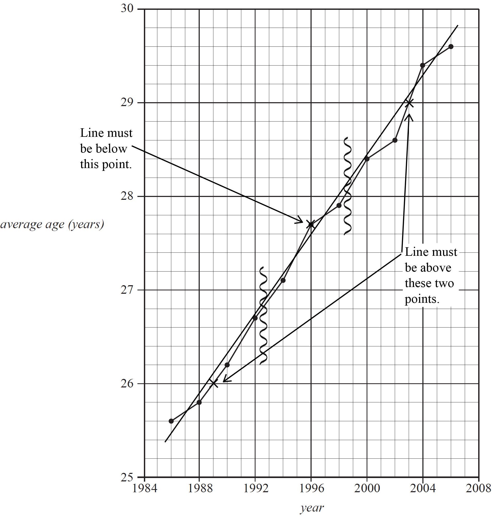
During the period 1986 to 2006, the average age of men at first marriage in a particular country indicated an increasing linear trend, as shown in the time plot below.

A three-median line could be used to model this trend.

On the graph above
i. clearly mark with a cross (×) the three points that would be used to fit a three-median line to this time series plot. (2 marks)

--- 0 WORK AREA LINES (style=lined) ---
ii. draw in the three-median line. (1 mark)

--- 0 WORK AREA LINES (style=lined) ---

Show Answers Only

`text(Constant between 1915 and 1935 and then)`
`text(decreasing between 1935 and 1970.)`

Show Worked Solution

a. `text(The average age of women at first marriage was fairly)`

`text(constant between 1915 and 1935, and then decreased)`

`text(between 1935 and 1970.)`

b.i. & ii.

CORE, FUR1 2010 VCAA 12 MC

The time series plot below shows the number of calls each month to a call centre over a twelve-month period.

The plot is to be smoothed using five-point median smoothing.

The smoothed number of calls for month number 10 is closest to

A. `358`

B. `364`

C. `371`

D. `375`

E. `377`

Show Answers Only

`D`

Show Worked Solution

`text(The median for the 5 values from month 8 – 12)`

♦ Mean mark 43%.

`text(is 40 calls.)`

`=> D`

CORE, FUR1 2015 VCAA 12 MC

The time series plot below charts the number of calls per year to a computer help centre over a 10-year period.

Using five-median smoothing, the smoothed number of calls in year 6 was closest to

A. `3500`

B. `3700`

C. `3800`

D. `4000`

E. `4200`

Show Answers Only

`D`

Show Worked Solution

`text(The median of the 5 data points from year 4 – year 8)`

`text(is 4000.)`

`=> D`

CORE, FUR1 2014 VCAA 13 MC

The time series plot below shows the hours of sunshine per day at a particular location for 16 consecutive days.

The three median method is used to fit a trend line to the data.

The slope of this trend line will be closest to

A. `–0.7`

B. `–0.2`

C. `0.0`

D. `0.2`

E. `0.7`

Show Answers Only

`C`

Show Worked Solution

`text(16 data points)`

♦ Mean mark 37%.

`text{Divide into 5, 6, 5 (3 groups)}`

`text(Median points for group)`

`text{Lower (3, 8)}`

`text{Upper (14, 8)}`

`text{Trend line from (3, 8) to (14, 8) is}`

`text(horizontal.)`

`∴\ text(Slope) = 0`

`=> C`

CORE, FUR1 2009 VCAA 13 MC

The time series plot below shows the growth in Internet use (%) in a country from 1989 to 1997 inclusive.

If a three-median line is fitted to the data it would show that, on average, the increase in Internet use per year was closest to

A. `0.33text(%)`

B. `0.36text(%)`

C. `0.41text(%)`

D. `0.45text(%)`

E. `0.49text(%)`

Show Answers Only

`D`

Show Worked Solution

`text(Median of 1989, 1990, 1991 = 0.6)`

♦ Mean mark 40%.
MARKERS’ COMMENT: Finding the slope of a three median line is a standard technique that many students clearly find difficult. Attention required.

`text(Median of 1995, 1996, 1997 = 3.3)`

`text(Average increase in median over 6 years)`