SmarterEd

Aussie Maths & Science Teachers: Save your time with SmarterEd

  • Login
  • Get Help
  • About

Data Analysis, GEN2 2024 NHT 4

In another study, the heights, in metres, of the highest high tide \(H H T\) for that day and the lowest low tide \(L L T\) for that day were recorded in Sydney Harbour for the 31 days of July 2021.

A scatterplot of this data is shown below.
 

When a least squares line is fitted to the scatterplot, the equation is found to be:

\(HHT=2.19-1.08 \times LLT\)

The coefficient of determination is 0.4709

  1. Draw the graph of the least squares line on the scatterplot above.   (1 mark)

    --- 0 WORK AREA LINES (style=lined) ---

  2. Determine the value of the correlation coefficient \(r\).
  3. Round your answer to three decimal places.   (1 mark)

    --- 1 WORK AREA LINES (style=lined) ---

  4. Describe the association between \(H H T\) and \(L L T\) in terms of form and direction.   (1 mark)

    --- 2 WORK AREA LINES (style=lined) ---

  5. Interpret the slope of the least squares line in terms of the variables \(H H T\) and \(L L T\).   (1 mark)

    --- 4 WORK AREA LINES (style=lined) ---

  6. In this investigation, the \(H H T\) value was 1.81 m for an \(L L T\) value of 0.40 m .
  7. Show that when this least squares line is fitted to the scatterplot, the residual for this point is 0.052    (2 marks)

    --- 4 WORK AREA LINES (style=lined) ---

  8. The mean of the \(H H T\) values for July 2021 is 1.70 m .
  9. Calculate the mean of the \(L L T\) values.
  10. Round your answer to two decimal places.    (1 mark)

    --- 5 WORK AREA LINES (style=lined) ---
Show Answers Only

a.


b.   \(r= -0.686\)

c.   \(\text{Form: Linear}\)

\(\text{Direction: Negative}\)

d.   \(\text{On average, when the \(LLT\) increases by 1.00 metre, the \(HHT\) decreases}\)

\(\text{by 1.08 metres.}\)

e.   \(\text{Actual values:}\ HHT=1.81\ \text{when}\ \ LLT=0.40 \)

\(\text{Predicted value}\ =2.19-1.08 \times 0.40 = 1.758\)

\(\text{Residual = Actual}-\text{Predicted}\ = 1.81-1.758=0.052\)
 

f.   \(LLT=0.45\)

Show Worked Solution

a.


b.
   \(r=-\sqrt{0.4709} = -0.686\)
 

c.   \(\text{Form: Linear}\)

\(\text{Direction: Negative}\)
 

d.   \(\text{Interpretation of slope:}\)

\(\text{On average, when the \(LLT\) increases by 1.00 metre, the \(HHT\) decreases}\)

\(\text{by 1.08 metres.}\)
 

e.   \(\text{Actual values:}\ HHT=1.81\ \text{when}\ \ LLT=0.40 \)

\(\text{Predicted value}\ =2.19-1.08 \times 0.40 = 1.758\)

\(\text{Residual = Actual}-\text{Predicted}\ = 1.81-1.758=0.052\)
 

f.   \(\text{Mean}\ (HHT)=1.70\)

\(1.70\) \(=2.19-1.08 \times LLT\)  
\(LLT\) \(=\dfrac{2.19-1.70}{1.08} = 0.45\ \text{(2 d.p.)}\)  

Filed Under: Correlation and Regression Tagged With: Band 3, Band 4, smc-265-30-LSRL formula, smc-265-40-Interpret Gradient, smc-265-50-Residuals

Data Analysis, GEN2 2024 VCAA 3

The Olympic gold medal-winning height for the women's high jump, \(\textit{Wgold}\), is often lower than the best height achieved in other international women's high jump competitions in that same year.

The table below lists the Olympic year, \(\textit{year}\), the gold medal-winning height, \(\textit{Wgold}\), in metres, and the best height achieved in all international women's high jump competitions in that same year, \(\textit{Wbest}\), in metres, for each Olympic year from 1972 to 2020.

A scatterplot of \(\textit{Wbest}\) versus \(\textit{Wgold}\) for this data is also provided.

When a least squares line is fitted to the scatterplot, the equation is found to be:

\(Wbest =0.300+0.860 \times Wgold\)

The correlation coefficient is 0.9318

  1. Name the response variable in this equation.   (1 mark)

    --- 1 WORK AREA LINES (style=lined) ---

  2. Draw the least squares line on the scatterplot above.  (1 mark)

    --- 0 WORK AREA LINES (style=lined) ---

  3. Determine the value of the coefficient of determination as a percentage.  (1 mark)
  4. Round your answer to one decimal place.

    --- 1 WORK AREA LINES (style=lined) ---

  5. Describe the association between \(\textit{Wbest}\) and \(\textit{Wgold}\) in terms of strength and direction.  (1 mark)

    --- 0 WORK AREA LINES (style=lined) ---

\begin{array}{|l|l|}
\hline
\rule{0pt}{2.5ex}\text { strength } \rule[-1ex]{0pt}{0pt} & \quad \quad\quad\quad\quad\quad\quad\quad\quad\quad\quad\\
\hline
\rule{0pt}{2.5ex}\text { direction } \rule[-1ex]{0pt}{0pt} & \\
\hline
\end{array}

  1. Referring to the equation of the least squares line, interpret the value of the slope in terms of the variables \(\textit{Wbest}\) and \(\textit{Wgold}\).  (1 mark)

    --- 3 WORK AREA LINES (style=lined) ---

  2. In 1984, the \(\textit{Wbest}\) value was 2.07 m for a \(\textit{Wgold}\) value of 2.02 m .
  3. Show that when this least squares line is fitted to the scatterplot, the residual value for this point is 0.0328.  (2 marks)

    --- 4 WORK AREA LINES (style=lined) ---

  4. The residual plot obtained when the least squares line was fitted to the data is shown below. The residual value from part f is missing from the residual plot.
     

    1. Complete the residual plot by adding the residual value from part f, drawn as a cross ( X ), to the residual plot above.   (1 mark)

      --- 0 WORK AREA LINES (style=lined) ---

    2. In part b, a least squares line was fitted to the scatterplot. Does the residual plot from part g justify this? Briefly explain your answer.  (1 mark)

      --- 3 WORK AREA LINES (style=lined) ---

  1. In 1964, the gold medal-winning height, \(\textit{Wgold}\), was 1.90m . When the least squares line is used to predict \(\textit{Wbest}\), it is found to be 1.934 m .
  2. Explain why this prediction is not likely to be reliable.  (1 mark)

    --- 2 WORK AREA LINES (style=lined) ---

Show Answers Only

a.    \(Wbest\)

b.    

c.    \(86.8\%\)

d.    \(\text{Strong, positive}\)

e.    \(Wbest\ \text{will increase, on average, by 0.86 metres for every metre of increase in}\ Wgold.\)

f.      \(Wbest\) \(=0.300 +0.86\times 2.02\)
    \(=2.0372\)

\(\therefore\ \text{Residual}\ =2.07-2.0372=0.0328\)

g.i.

g.ii.  \(\text{Yes, it is justified as there is no clear pattern, linear or otherwise.}\)

h.    \(\text{This prediction is outside the data range (1972 – 2020 → extrapolation)}\)

\(\text{and therefore cannot be relied upon.}\)

Show Worked Solution

a.    \(Wbest\)

b.    \(\text{Using points:}\ (1.90, 1.934)\ \text{and}\ (2.00, 2.02)\)
 

Mean mark (b) 51%.

c.    \(r=0.9318\ \ \Rightarrow\ \ r^2=0.9318^2=0.8682\dots\)

\(\therefore\ \text{Coefficient of determination} \approx 86.8\%\)
 

d.    \(\text{Strong, positive}\)
 

e.    \(Wbest\ \text{will increase, on average, by 0.86 metres for every metre of increase in}\ Wgold.\)
 

f.      \(Wbest\) \(=0.300 +0.86\times 2.02\)
    \(=2.0372\)

 
\(\therefore\ \text{Residual}\ =2.07-2.0372=0.0328\)

♦ Mean mark (f) 48%.

g.i.

g.ii.  \(\text{Yes, it is justified as there is no clear pattern, linear or otherwise.}\)

♦ Mean mark (g)(i) 47%.
♦ Mean mark (g)(ii) 40%.

h.    \(\text{This prediction is outside the data range (1972–2020 → extrapolation)}\)

\(\text{and therefore cannot be relied upon.}\)

♦ Mean mark (h) 50%.

Filed Under: Correlation and Regression Tagged With: Band 3, Band 4, Band 5, smc-265-10-r / r^2 and Association, smc-265-30-LSRL formula, smc-265-40-Interpret Gradient, smc-265-50-Residuals, smc-265-60-Extrapolation / Interpolation, smc-265-75-Explanatory / Response

Data Analysis, GEN1 2022 VCAA 7-8 MC

The association between the weight of a seal's spleen, spleen weight, in grams, and its age, in months, for a sample of seals is non-linear.

This association can be linearised by applying a \(\log _{10}\) transformation to the variable spleen weight.
 

The equation of the least squares line for this scatterplot is

\(\log _{10}\) (spleen weight) = 2.698 + 0.009434 × age

 
Question 7

The equation of the least squares line predicts that, on average, for each one-month increase in the age of the seals, the increase in the value of \(\log _{10}\) (spleen weight) is

  1. 0.009434
  2. 0.01000
  3. 1.020
  4. 2.698
  5. 5.213

 
Question 8

Using the equation of the least squares line, the predicted spleen weight of a 30-month-old seal, in grams, is

  1. 3
  2. 511
  3. 772
  4. 957
  5. 1192
Show Answers Only

\(\text{Question 7:} \ A\)

\(\text{Question 8:} \ D\)

Show Worked Solution

\(\text{Question 7}\)

\(\text{Graph passes through (0, 2.7) and (130, 3.93)} \)

\(\text{Gradient}\ \approx \dfrac{3.93-2.7}{130} \approx 0.0946 \)

\(\Rightarrow A\)
 

\(\text{Question 8}\)

\(\text{Let the predicted spleen weight be}\ w:\)

\(\log_{10} w\) \(=2.698 + 0.009434 \times 30\)  
\(\log_{10} w\) \(=2.98102\)  
\(w\) \(= 10^{2.98102}\)  
  \(=957.2381527\)  

 
\(\Rightarrow D\)

Mean mark (Q8) 56%.

Filed Under: Correlation and Regression Tagged With: Band 4, smc-265-30-LSRL formula, smc-265-40-Interpret Gradient, smc-265-70-Linearise - log10

CORE, FUR2 2021 VCAA 3

The time series plot below shows the winning time, in seconds, for the women's 100 m freestyle swim plotted against year, for each year that the Olympic Games were held during the period 1956 to 2016.

A least squares line has been fitted to the plot to model the decreasing trend in the winning time over this period.
 

The equation of the least squares line is

winning time = 357.1 – 0.1515 × year

The coefficient of determination is 0.8794

  1. Name the explanatory variable in this time series plot.   (1 mark)

    --- 1 WORK AREA LINES (style=lined) ---

  2. Determine the value of the correlation coefficient (`r`).
  3. Round your answer to three decimal places.   (1 mark)

    --- 2 WORK AREA LINES (style=lined) ---

  4. Write down the average decrease in winning time, in seconds per year, during the period 1956 to 2016.   (1 mark)

    --- 2 WORK AREA LINES (style=lined) ---

  5. The predicted winning time for the women's 100 m freestyle in 2000 was 54.10 seconds.
  6. The actual winning time for the women's 100 m freestyle in 2000 was 53.83 seconds.
  7. Determine the residual value in seconds.   (1 mark)

    --- 2 WORK AREA LINES (style=lined) ---

  8. The following equation can be used to predict the winning time for the women's 100 m freestyle in the future.
  9.      winning time =  357.1 – 0.1515 × year
  10.  i. Show that the predicted winning time for the women's 100 m freestyle in 2032 is 49.252 seconds.   (1 mark)

    --- 2 WORK AREA LINES (style=lined) ---

  11. ii. What assumption is being made when this equation is used to predict the winning time for the women's 100 m freestyle in 2032?   (1 mark)

    --- 2 WORK AREA LINES (style=lined) ---

Show Answers Only
  1. `text{year}`
  2. `- 0.938`
  3. `0.1515 \ text{seconds}`
  4. `-0.27`
  5.  i. `49.252 \ text{seconds}`
  6. ii. `text{The same trend continues when the graph is extended beyond 2016.}`
Show Worked Solution

a.      `text{year}`
 

b. `r^2` `= 0.8794 \ text{(given)}`
  `r` `= ± sqrt{0.8794}`
    `= ± 0.938 \ text{(to 3 d.p.)}`

 
`text{By inspection of graph, correlation is negative}`

`:. \ r = -0.938`
 

c.    `text{Average decrease in winning time = 0.1515 seconds}`

`text{(this is given by the slope of the line.)}`
 

d.    `text{Residual Value}` `= text{actual}-text{predicted}`
    `= 53.83-54.10`
    `= -0.27`


e.i.      `text{winning time (2032)}` `= 357.1-0.1515 xx 2032`
      `=49.252 \ text{seconds}`


e.ii.  `text{The assumption is that the graph is accurate when it is extended}`

  `text{beyond 2016 (i.e decreasing trend continues).}`

Filed Under: Correlation and Regression Tagged With: Band 3, Band 4, Band 5, smc-265-10-r / r^2 and Association, smc-265-30-LSRL formula, smc-265-40-Interpret Gradient, smc-265-50-Residuals, smc-265-60-Extrapolation / Interpolation, smc-265-75-Explanatory / Response

CORE, FUR2 2020 VCAA 5

The scatterplot below shows body density, in kilograms per litre, plotted against waist measurement, in centimetres, for 250 men.

When a least squares line is fitted to the scatterplot, the equation of this line is

body density = 1.195 – 0.001512 × waist measurement

  1. Draw the graph of this least squares line on the scatterplot above.   (1 mark)

    --- 0 WORK AREA LINES (style=lined) ---

  2. Use the equation of this least squares line to predict the body density of a man whose waist measurement is 65 cm.
  3. Round your answer to two decimal places.   (1 mark)

    --- 2 WORK AREA LINES (style=lined) ---

  4. When using the equation of this least squares line to make the prediction in part b., are you extrapolating or interpolating?   (1 mark)

    --- 1 WORK AREA LINES (style=lined) ---

  5. Interpret the slope of this least squares line in terms of a man’s body density and waist measurement.   (1 mark)

    --- 2 WORK AREA LINES (style=lined) ---

  6. In this study, the body density of the man with a waist measurement of 122 cm was 0.995 kg/litre.
  7. Show that, when this least squares line is fitted to the scatterplot, the residual, rounded to two decimal places, is –0.02   (1 mark)

    --- 3 WORK AREA LINES (style=lined) ---

  8. The coefficient of determination for this data is 0.6783
  9. Write down the value of the correlation coefficient `r`.
  10. Round your answer to three decimal places.   (1 mark)

    --- 2 WORK AREA LINES (style=lined) ---

  11. The residual plot associated with fitting a least squares line to this data is shown below.


    Does this residual plot support the assumption of linearity that was made when fitting this line to this data? Briefly explain your answer.   (1 mark)

    --- 3 WORK AREA LINES (style=lined) ---

Show Answers Only
  1. `text(See Worked Solutions)`
  2. `1.10\ text(kg/litre)`
  3. `text(extrapolating)`
  4. `text(See Worked Solutions)`
  5. `-0.02`
  6. `-0.824`
  7. `text(See Worked Solutions)`
Show Worked Solution

a.   `text(LSRL passes through)\ (60, 1.1043) and (130, 0.998)`

♦ Mean mark part a. 41%.

b.   `text(body density)` `= 1.195-0.001512 xx 65`
    `= 1.09672`
    `= 1.10\ text{kg/litre (to 2 d.p.)}`
♦ Mean mark part c. 38%.
c.   `text(A waist of 65 cm is outside the)`
  `text(range of the existing data set.)`

 
`:.\ text(Extrapolating)`


♦ Mean mark part d. 44%.
d.   `text(Body density decreases by 0.001512 kg/litre)`
  `text(for each increase in waist size of 1 cm.)`


e.   `text{Body density (predicted)}`

`= 1.195-0.001512 xx 122`

`~~ 1.0105\ text(kg/litre)`
 

`text(Residual)` `= text(Actual-predicted)`
  `~~ 0.995-1.0105`
  `~~ -0.0155`
  `~~ -0.02\ text{(to 2 d.p.)}`


♦♦ Mean mark part f. 25%.

f.   `r` `= -sqrt(0.6783)`
    `=-0.8235…`
    `= -0.824\ text{(to 3 d.p.)}`


g.  `text(The residual plot has no pattern and is centred around zero.)`

`:.\ text(It supports the assumption of linearity of the LSRL.)`

Filed Under: Correlation and Regression Tagged With: Band 4, Band 5, smc-265-10-r / r^2 and Association, smc-265-30-LSRL formula, smc-265-40-Interpret Gradient, smc-265-50-Residuals, smc-265-60-Extrapolation / Interpolation

Data Analysis, GEN2 2019 NHT 4

The scatterplot below plots the variable life span, in years, against the variable sleep time, in hours, for a sample of 19 types of mammals.
 

On the assumption that the association between sleep time and life span is linear, a least squares line is fitted to this data with sleep time as the explanatory variable.

The equation of this least squares line is

life span = 42.1 – 1.90 × sleep time

The coefficient of determination is 0.416

  1. Draw the graph of the least squares line on the scatterplot above.   (1 mark)

    --- 0 WORK AREA LINES (style=lined) ---

  2. Describe the linear association between life span and sleep time in terms of strength and direction.   (2 marks)

    --- 2 WORK AREA LINES (style=lined) ---

  3. Interpret the slope of the least squares line in terms of life span and sleep time.   (2 marks)

    --- 2 WORK AREA LINES (style=lined) ---

  4. Interpret the coefficient of determination in terms of life span and sleep time.   (1 mark)

    --- 2 WORK AREA LINES (style=lined) ---

  5. The life of the mammal with a sleep time of 12 hours is 39.2 years.
  6. Show that, when the least squares line is used to predict the life span of this mammal, the residual is 19.9 years.   (2 marks)

    --- 4 WORK AREA LINES (style=lined) ---

Show Answers Only
  1.  

  2. `text(Strength is moderate.)`


    `text(Direction is negative.)`

  3. `text(The gradient of –1.9 means that life span decreases by)` 


    `text(1.9 years for each additional hour of sleep time.)`

  4. `text(41.6% of the variation in life span can be explained by the)`


    `text(variation in sleep time.)`

  5. `text(Proof(See Worked Solution))`
Show Worked Solution

a.    `text{Graph endpoints (0, 42.1) and (18, 7.9)}`


b.   `text(Strength is moderate.)`

`text(Direction is negative.)`
 

c.    `text(The gradient of –1.9 means that life span decreases by)`

`text(1.9 years for each additional hour of sleep time.)`


d.    `text(41.6% of the variation in life span can be explained by the )`

`text(variation in sleep time.)`
 

e.    `text(Predicted value)` `= 42.1 – 1.9 xx 12`
  `= 19.3 \ text(years)`


`text(Residual)` `= text(actual) – text(predicted)`
  `= 39.2 – 19.3`
  `= 19.9 \ text(years)`

Filed Under: Correlation and Regression Tagged With: Band 3, Band 4, Band 5, smc-265-10-r / r^2 and Association, smc-265-40-Interpret Gradient, smc-265-50-Residuals

CORE, FUR2 2019 VCAA 5

The scatterplot below shows the atmospheric pressure, in hectopascals (hPa), at 3 pm (pressure 3 pm) plotted against the atmospheric pressure, in hectopascals, at 9 am (pressure 9 am) for 23 days in November 2017 at a particular weather station.
 

A least squares line has been fitted to the scatterplot as shown.

The equation of this line is

pressure 3 pm = 111.4 + 0.8894 × pressure 9 am

  1. Interpret the slope of this least squares line in terms of the atmospheric pressure at this weather station at 9 am and at 3 pm.   (1 mark)

    --- 2 WORK AREA LINES (style=lined) ---

  2. Use the equation of the least squares line to predict the atmospheric pressure at 3 pm when the atmospheric pressure at 9 am is 1025 hPa.
  3. Round your answer to the nearest whole number.   (1 mark)

    --- 2 WORK AREA LINES (style=lined) ---

  4. Is the prediction made in part b. an example of extrapolation or interpolation?   (1 mark)

    --- 1 WORK AREA LINES (style=lined) ---

  5. Determine the residual when the atmospheric pressure at 9 am is 1013 hPa.
  6. Round your answer to the nearest whole number.   (1 mark)

    --- 3 WORK AREA LINES (style=lined) ---

  7. The mean and the standard deviation of pressure 9 am and pressure 3 pm for these 23 days are shown in Table 4 below.

    1. Use the equation of the least squares line and the information in Table 4 to show that the correlation coefficient for this data, rounded to three decimal places, is  `r` = 0.966   (1 mark)

      --- 3 WORK AREA LINES (style=lined) ---

    2. What percentage of the variation in pressure 3 pm is explained by the variation in pressure 9 am?
    3. Round your answer to one decimal place.   (1 mark)

      --- 2 WORK AREA LINES (style=lined) ---

  1. The residual plot associated with the least squares line is shown below.
     

    1. The residual plot above can be used to test one of the assumptions about the nature of the association between the atmospheric pressure at 3 pm and the atmospheric pressure at 9 am.
    2. What is this assumption?   (1 mark)

      --- 2 WORK AREA LINES (style=lined) ---

    3. The residual plot above does not support this assumption.
    4. Explain why.   (1 mark)

      --- 2 WORK AREA LINES (style=lined) ---

Show Answers Only
  1. `text(An increase in 1hPa of pressure at 9 am is associated)`
    `text(with an increase of 0.8894 hPa of pressure at 3 pm.)`
  2. `1023\ text(hPa)`
  3. `text(Interpolation)`
  4. `3\ text(hPa)`
    1. `0.966`
    2. `93.3%`
    1. `text(The assumption is that a linear relationship)`
      `text(exists between the pressure at 9 am and the)`
      `text(pressure at 3 pm.)`
    2. `text(The residual plot does not appear to be random.)`
Show Worked Solution

a.    `text(An increase in 1hPa of pressure at 9 am is associated)`

`text(with an increase of 0.8894 hPa of pressure at 3 pm.)`


b.   `text(pressure 3 pm)` `= 111.4 + 0.8894 xx 1025`
    `= 1023\ text(hPa)`


c.  `text{Interpolation (1025 is within the given data range)}`


d.   `text(Residual)` `= text(actual) – text(predicted)`
    `= 1015 – (111.4 + 0.8894 xx 1013)`
    `= 1015 – 1012.36`
    `= 2.63…`
    `~~ 3\ text(hPa)`


e.i.   `r= b (s_x)/(s_y)`

    `= 0.8894 xx 4.5477/4.1884`
    `= 0.96569…`
    `= 0.966`


e.ii.   `r` `= 0.966`
  `r^2` `= 0.9331`
    `= 93.3%`


f.i.   `text(The assumption is that a linear relationship)`
 

`text(exists between the pressure at 9 am and the)`

`text(pressure at 3 pm.)`


f.ii.  `text(The residual plot does not appear to be random.)`

Filed Under: Correlation and Regression Tagged With: Band 3, Band 4, Band 5, page-break-before-question, smc-265-10-r / r^2 and Association, smc-265-30-LSRL formula, smc-265-40-Interpret Gradient, smc-265-50-Residuals, smc-265-60-Extrapolation / Interpolation

CORE, FUR1 2019 VCAA 11 MC

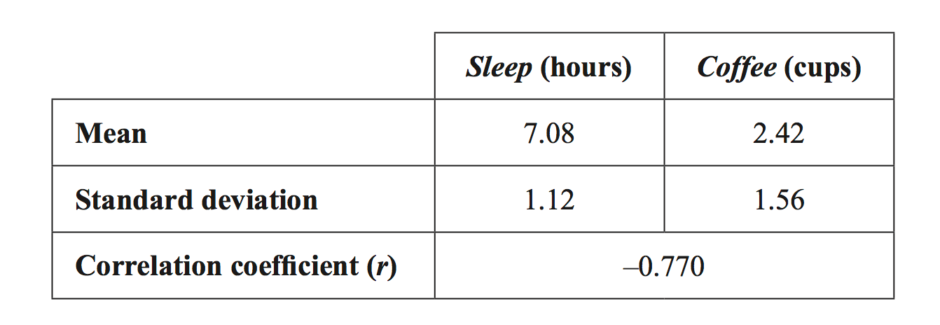
A study was conducted to investigate the effect of drinking coffee on sleep.

In this study, the amount of sleep, in hours, and the amount of coffee drunk, in cups, on a given day were recorded for a group of adults.

The following summary statistics were generated.

On average, for each additional cup of coffee drunk, the amount of sleep

  1. decreased by 0.55 hours.
  2. decreased by 0.77 hours.
  3. decreased by 1.1 hours.
  4. increased by 1.1 hours.
  5. increased by 2.3 hours.
Show Answers Only

`A`

Show Worked Solution
`b` `= r xx (s_y)/(s_x)`
  `= -0.770 xx 1.12/1.56`
  `= -0.55\ text(hours)`

 
`:.\ text(Sleep decreased by 0.55 hours for each)`

`text(additional cup of coffee.)`

`=>  A`

Filed Under: Correlation and Regression Tagged With: Band 5, smc-265-30-LSRL formula, smc-265-40-Interpret Gradient

CORE, FUR1 2018 VCAA 14 MC

A least squares line is fitted to a set of bivariate data.

Another least squares line is fitted with response and explanatory variables reversed.

Which one of the following statistics will not change in value?

  1. the residual values
  2. the predicted values
  3. the correlation coefficient `r`
  4. the slope of the least squares line
  5. the intercept of the least squares line
Show Answers Only

`C`

Show Worked Solution

`text(If the variables are reversed, the equation changes.)`

♦ Mean mark 42%.

`:.\ text(Differences will occur in:)`

`text(- slope)`

`text(- intercept)`

`text(- predicted and residual values)`
 

`text(The correlation co-efficient will remain unchanged however,)`

`text(as the scattering of the points around the line of best fit is)`

`text{the same (i.e. scattering of}\ x\ text(values relative to)\ y\ text(values)`

`text(is the same as)\ y\ text(values relative to)\ x).`

`=> C`

Filed Under: Correlation and Regression Tagged With: Band 5, smc-265-10-r / r^2 and Association, smc-265-40-Interpret Gradient, smc-265-50-Residuals, smc-265-75-Explanatory / Response

CORE, FUR1 2018 VCAA 10 MC

In a study of the association between a person’s height, in centimetres, and body surface area, in square metres, the following least squares line was obtained.

body surface area = –1.1 + 0.019 × height

Which one of the following is a conclusion that can be made from this least squares line?

  1. An increase of 1 m² in body surface area is associated with an increase of 0.019 cm in height.
  2. An increase of 1 cm in height is associated with an increase of 0.019 m² in body surface area.
  3. The correlation coefficient is 0.019
  4. A person’s body surface area, in square metres, can be determined by adding 1.1 cm to their height.
  5. A person’s height, in centimetres, can be determined by subtracting 1.1 from their body surface area, in square metres.
Show Answers Only

`B`

Show Worked Solution

`text(By definition of the equation, option)\ B\ text(is a)`

♦ Mean mark 51%.

`text(correct conclusion.)`

`=> B`

Filed Under: Correlation and Regression Tagged With: Band 4, smc-265-40-Interpret Gradient

CORE, FUR2 2017 VCAA 3

The number of male moths caught in a trap set in a forest and the egg density (eggs per square metre) in the forest are shown in the table below.
 

  1. Determine the equation of the least squares line that can be used to predict the egg density in the forest from the number of male moths caught in the trap.
  2. Write the values of the intercept and slope of this least squares line in the appropriate boxes provided below.
  3. Round your answers to one decimal place.  (2 marks)

    --- 0 WORK AREA LINES (style=lined) ---


  4. The number of female moths caught in a trap set in a forest and the egg density (eggs per square metre) in the forest can also be examined.


    A scatterplot of the data is shown below.


    The equation of the least squares line is


                  egg density = 191 + 31.3 × number of female moths

    1. Draw the graph of this least squares line on the scatterplot (provided above).   (1 mark)

      --- 0 WORK AREA LINES (style=lined) ---

    2. Interpret the slope of the regression line in terms of the variables egg density and number of female moths caught in the trap.   (1 mark)

      --- 2 WORK AREA LINES (style=lined) ---

    3. The egg density is 1500 when the number of female moths caught is 55.
    4. Determine the residual value if the least squares line is used to predict the egg density for this number of female moths.   (1 mark)

      --- 3 WORK AREA LINES (style=lined) ---

    5. The correlation coefficient is  `r = 0.862`
    6. Determine the percentage of the variation in egg density in the forest explained by the variation in the number of female moths caught in the trap.
    7. Round your answer to one decimal place.   (1 mark)

      --- 3 WORK AREA LINES (style=lined) ---

Show Answers Only

a.   `text(egg density)\ = −46.8 + 18.9 xx text(number of male moths)`

b.i.  

b.ii.  `text(Egg density per square metre increases)`

`text(by 31.3 eggs for every extra female moth)`

`text(caught in the trap.)`

b.iii.  `−412.5`

b.iv.  `text(74.3%)`

Show Worked Solution

a.   `text(By calculator)`

`text(egg density)\ = −46.8 + 18.9 xx text(number of male moths)`


b.i.   `text(Calculating extreme points on graph.)`

♦♦ Mean mark 26%.
MARKER’S COMMENT: Not well answered! Many students did not realise the graph started at 10 on the `x`-axis and many did not use a ruler!

`x = 10, y = 191 + 31.3 xx 10 = 504`

`x = 60, y = 191 + 31.3 xx 60 = 2069`


♦ Mean mark 39%.
MARKER’S COMMENT: Students must clearly refer to the increase in egg density for every one-unit increase in female moths.

b.ii.   `text(Egg density per square metre increases)`

 `text(by 31.3 eggs for every extra female moth)`

 `text(caught in the trap.)`


b.iii.   `text(Predicted egg density)`

♦ Mean mark 48%.

`= 191 + 31.3 xx 55`

`= 1912.5`

`:.\ text(Residual value)` `= 1500-1912.5`
  `= −412.5`


b.iv.   `r = 0.862`

♦ Mean mark 47%.

`r^2 = 0.862^2 = 0.7430… = 74.3text{%  (1 d.p.)}`

`:.\ text(74.3% is explained.)`

Filed Under: Correlation and Regression Tagged With: Band 4, Band 5, smc-265-10-r / r^2 and Association, smc-265-20-Find LSRL Equation/Gradient, smc-265-40-Interpret Gradient, smc-265-50-Residuals

CORE, FUR2 2006 VCAA 2

The heights (in cm) and ages (in months) of a random sample of 15 boys have been plotted in the scatterplot below. The least squares regression line has been fitted to the data.


The equation of the least squares regression line is 

`text(height = 75.4 + 0.53 × age)`

The correlation coefficient is  `r= 0.7541`

  1. Complete the following sentence.


    On average, the height of a boy increases by _______ cm for each one-month increase in age.   (1 mark)

    --- 0 WORK AREA LINES (style=lined) ---

  2.  i. Evaluate the coefficient of determination.
  3.     Write your answer, as a percentage, correct to one decimal place.   (1 mark)

    --- 1 WORK AREA LINES (style=lined) ---

  4. ii. Interpret the coefficient of determination in terms of the variables height and age.   (1 mark)

    --- 2 WORK AREA LINES (style=lined) ---

Show Answers Only

a.    `0.53`

b.i.   `text(56.9%)`

b.ii. `text{The coefficient of determination 0.569 (56.9%) represents}`

`text{the proportion (percentage) of the variability in height with age}`

`text(that is explained by the least squares regression line.)`

Show Worked Solution

a.   `0.53`

♦ Average mean mark for all parts 44%.
MARKER’S COMMENT: b.i. errors included not converting to % and rounding as a decimal before converting and answering 60%.


b.i.    `r^2` `= 0.7541^2`
    `= 0.5686…`
    `= 56.9text(%)`
MARKER’S COMMENT: Any reference to causation in b.ii. was marked incorrect.


b.ii.  `text{56.9% of the variation in height is}`

`text{explained by the variation in age.}`

Filed Under: Correlation and Regression Tagged With: Band 4, Band 5, smc-265-10-r / r^2 and Association, smc-265-40-Interpret Gradient

CORE, FUR2 2007 VCAA 2

The mean surface temperature (in °C) of Australia for the period 1960 to 2005 is displayed in the time series plot below.

2007 2-1

  1. In what year was the lowest mean surface temperature recorded?   (1 mark)

    --- 1 WORK AREA LINES (style=lined) ---

The least squares method is used to fit a trend line to the time series plot.

  1.   i. The equation of this trend line is found to be
  2.          mean surface temperature = – 12.361 + 0.013 × year
  3.      Use the trend line to predict the mean surface temperature (in °C) for 2010.
  4.      Write your answer correct to two decimal places.   (1 mark)

    --- 1 WORK AREA LINES (style=lined) ---

  5.  ii. The actual mean surface temperature in the year 2000 was 13.55°C.
  6.      Determine the residual value (in °C) when the trend line is used to predict the mean surface temperature for this year.
  7.      Write your answer correct to two decimal places.   (1 mark)

    --- 3 WORK AREA LINES (style=lined) ---

  8. iii. By how many degrees does the trend line predict Australia's mean surface temperature will rise each year?
  9.      Write your answer correct to three decimal places.   (1 mark)

    --- 2 WORK AREA LINES (style=lined) ---

Show Answers Only
  1. `1964`
    1. `13.77 text(°C)`
    2. `-0.09`
    3. `0.013 text(°C)`
Show Worked Solution

a.   `1964`
 

b.i.   `text{Mean surface temperature (2010)}`

`= -12.361 + 0.013 xx 2010`

`=13.769`

`= 13.77 text{°C  (2 d.p.)}`
 

b.ii.   `text{Predicted mean surface temp (2010)}`

MARKER’S COMMENT: A common error was to omit the negative sign.

`= -12.361 + 0.013 xx 2000`

`= 13.639 text(°C)`


`:.\ text(Residual)` `= 13.55-13.639`
  `= -0.089`
  `=-0.09\ text{(2 d.p.)}`


b.iii.   `text(S)text(ince the gradient of the equation = 0.013,)`

  `text(the temperature is predicted to rise 0.013°C)`

  `text(each year.)`

Filed Under: Correlation and Regression Tagged With: Band 3, Band 4, smc-265-40-Interpret Gradient, smc-265-50-Residuals

CORE, FUR2 2008 VCAA 4

The arm spans (in cm) and heights (in cm) for a group of 13 boys have been measured. The results are displayed in the table below.
 

CORE, FUR2 2008 VCAA 4 

The aim is to find a linear equation that allows arm span to be predicted from height.

  1. What will be the explanatory variable in the equation?   (1 mark)

    --- 1 WORK AREA LINES (style=lined) ---

  2. Assuming a linear association, determine the equation of the least squares regression line that enables arm span to be predicted from height. Write this equation in terms of the variables arm span and height. Give the coefficients correct to two decimal places.   (2 marks)

    --- 2 WORK AREA LINES (style=lined) ---

  3. Using the equation that you have determined in part b., interpret the slope of the least squares regression line in terms of the variables height and arm span.   (1 mark)

    --- 2 WORK AREA LINES (style=lined) ---

Show Answers Only
  1. `text(Height)`
  2. `text(Arm span)\ = 1.09 xx text(height) – 15.63`
  3. `text(On average, arm span increases by 1.09 cm)`


    `text(for each 1 cm increase in height.)`

Show Worked Solution

a.   `text(Height)`

♦ Mean mark sub 50% (exact data not available).
MARKER’S COMMENT: Many students did not understand the term co-efficients as it applies to the regression equation.


b.   `text(By calculator,)`

`text(Arm span)\ = 1.09 xx text(height) – 15.63`


c.   `text(On average, arm span increases by 1.09 cm)`

`text(for each 1 cm increase in height.)`

Filed Under: Correlation and Regression Tagged With: Band 4, Band 5, smc-265-20-Find LSRL Equation/Gradient, smc-265-40-Interpret Gradient, smc-265-75-Explanatory / Response

CORE, FUR2 2010 VCAA 2

In the scatterplot below, average annual female income, in dollars, is plotted against average annual male income, in dollars, for 16 countries. A least squares regression line is fitted to the data.


The equation of the least squares regression line for predicting female income from male income is

female income = 13 000 + 0.35 × male income

  1. What is the explanatory variable?  (1 mark)

    --- 1 WORK AREA LINES (style=lined) ---

  2. Complete the following statement by filling in the missing information.


    From the least squares regression line equation it can be concluded that, for these countries, on average, female income increases by `text($________)` for each $1000 increase in male income.  (1 mark)

    --- 0 WORK AREA LINES (style=lined) ---

    1. Use the least squares regression line equation to predict the average annual female income (in dollars) in a country where the average annual male income is $15 000.  (1 mark)

      --- 1 WORK AREA LINES (style=lined) ---

    2. The prediction made in part c.i. is not likely to be reliable.


      Explain why.  (1 mark)

      --- 2 WORK AREA LINES (style=lined) ---


Show Answers Only

  1. `text(Male income)`
  2. `$350`
    1. `$18\ 250`
    2. `text(The model established by the regression)`
      `text(equation cannot be relied upon outside the)`
      `text(range of the given data set.)`
  3.  

Show Worked Solution

a.   `text(Male income)`
 

b.   `text(Increase in female income)`

`= 0.35 xx 1000`

`= $350`
 

c.i.   `text(Average annual female income)`

`= 13\ 000 + 0.35 xx 15\ 000`

`= $18\ 250`

♦♦ This part was poorly answered (exact data unavailable).
MARKER’S COMMENT: Many students offered “real world” explanations which did not gain a mark here.

 
c.ii.
   `text(The model established by the regression)`

   `text(equation cannot be relied upon outside the)`

   `text(range of the given data set.)`

Filed Under: Correlation and Regression Tagged With: Band 3, Band 4, Band 5, smc-265-40-Interpret Gradient, smc-265-60-Extrapolation / Interpolation, smc-265-75-Explanatory / Response

CORE, FUR2 2012 VCAA 2

The maximum temperature and the minimum temperature at this weather station on each of the 30 days in November 2011 are displayed in the scatterplot below.

CORE, FUR2 2012 VCAA 2

The correlation coefficient for this data set is  `r = 0.630`. 

The equation of the least squares regression line for this data set is

maximum temperature = `13 + 0.67` × minimum temperature

  1. Draw this least squares regression line on the scatterplot above.   (1 mark)

    --- 0 WORK AREA LINES (style=lined) ---

  2. Interpret the vertical intercept of the least squares regression line in terms of maximum temperature and minimum temperature.   (1 mark)

    --- 2 WORK AREA LINES (style=lined) ---

  3. Describe the relationship between the maximum temperature and the minimum temperature in terms of strength and direction.   (1 mark)

    --- 2 WORK AREA LINES (style=lined) ---

  4. Interpret the slope of the least squares regression line in terms of maximum temperature and minimum temperature.   (1 mark)

    --- 2 WORK AREA LINES (style=lined) ---

  5. Determine the percentage of variation in the maximum temperature that may be explained by the variation in the minimum temperature.
  6. Write your answer, correct to the nearest percentage.   (1 mark)

    --- 2 WORK AREA LINES (style=lined) ---

On the day that the minimum temperature was 11.1 °C, the actual maximum temperature was 12.2 °C.

  1. Determine the residual value for this day if the least squares regression line is used to predict the maximum temperature.
  2. Write your answer, correct to the nearest degree.   (2 marks)

    --- 4 WORK AREA LINES (style=lined) ---

Show Answers Only
  1. `text(See Worked Solutions)`
  2. `text(On average, when the minimum temperature is)`
    `text(0 °C, the maximum temperature is 13 °C)`
  3. `text(Moderate and positive.)`
  4. `text(On average, it is predicted that the maximum)`
    `text(temperature increases by 0.67 °C for every 1 °C)`
    `text(increase in the minimum temperature.)`
  5. `40text(%)`
  6. `-8^@text(C)`
Show Worked Solution

a.   `text(The two widest points in this data range are,)`

`text{(0, 13) and (20, 26.4).}`

 CORE, FUR2 2012 VCAA 2 Answer 

b.   `text(On average, when the minimum temperature is)`

`text(0 °C, the maximum temperature is 13 °C.)`


♦ Parts (i) to (vi) have an average mean mark of 41%.

c.   `text(Given)\ r = 0.630,`

`text(Strength: moderate)`

`text(Direction: positive)`


d.   `text(On average, it is predicted that \the maximum)`

 `text(temperature increases by 0.67 °C for every 1 °C)`

 `text(increase in the minimum temperature.)`


e.    `r^2` `= 0.630^2`
    `=0.3969`
    `=40text{%  (nearest %)}`


f.   `text(When the minimum temperature was)\ 11.1 text(°C),`

MARKER’S COMMENT: Students had particular difficulty with this part, with many using the incorrect calculation of  12.2 – 11.1 = 1.1.
`text(Predicted Value)` `= 13 + 0.67 xx 11.1`
  `=20.437…`
`:.\ text(Residual)` `= 12.2 − 20.437…`
  `= – 8.237…`
  `= – 8\ text{°C (nearest degree)}`

Filed Under: Correlation and Regression Tagged With: Band 4, Band 5, Band 6, smc-265-10-r / r^2 and Association, smc-265-40-Interpret Gradient, smc-265-50-Residuals

CORE, FUR2 2014 VCAA 2

The scatterplot below shows the population and area (in square kilometres) of a sample of inner suburbs of a large city.
 

Core, FUR2 2015 VCAA 2

The equation of the least squares regression line for the data in the scatterplot is

population = 5330 + 2680 × area

  1. Write down the response variable.   (1 mark)

    --- 1 WORK AREA LINES (style=lined) ---

  2. Draw the least squares regression line on the scatterplot above.   (1 mark)

    --- 0 WORK AREA LINES (style=lined) ---

  3. Interpret the slope of this least squares regression line in terms of the variables area and population.  (2 marks)

    --- 4 WORK AREA LINES (style=lined) ---

  4. Wiston is an inner suburb. It has an area of 4 km² and a population of 6690.
  5. The correlation coefficient, `r`, is equal to 0.668
  6.  i. Calculate the residual when the least squares regression line is used to predict the population of Wiston from its area.  (1 mark)

    --- 2 WORK AREA LINES (style=lined) ---

  7. ii. What percentage of the variation in the population of the suburbs is explained by the variaton in area.
  8.     Write your answer, correct to one decimal place.  (1 mark)

    --- 2 WORK AREA LINES (style=lined) ---

Show Answers Only
  1. `text(Population.)`
  2.  
          Core, FUR2 2015 VCAA 2 Answer
  3. `text(Population increases by 2680 people, on average,)`
    `text(for each additional 1 km² in area.)`
    1. ` −9360`
    2. `text(44.6%)`
Show Worked Solution

a.   `text(Population.)`
 

♦ Mean mark 36%.
MARKER’S COMMENT: Use the equation to draw the line and use points at the extremities.
b.   

Core, FUR2 2015 VCAA 2 Answer


c.   `text(Population increases by 2680 people, on average,)`

♦ Mean mark 41% (part (iii)).

`text(for each additional 1 km² in area.)`
 

d.i.  `text(Predicted population) = 5330 + 2680 xx 4= 16\ 050`

`:.\ text(Residual)\ = 6690-16\ 050= -9360`
 

♦ Part (iv) in total had a mean mark 42%.
d.ii.    `r` `= 0.668^2`
  `r^2` `= 0.4462…`
    `= 44.6 text{%  (to 1 d.p.)}`


`:.\ text(44.6% of the variation in the population is explained)`

`text(by variation in the area.)`

Filed Under: Correlation and Regression Tagged With: Band 4, Band 5, smc-265-10-r / r^2 and Association, smc-265-40-Interpret Gradient, smc-265-75-Explanatory / Response

CORE, FUR2 2015 VCAA 3

The scatterplot below plots male life expectancy (male) against female life expectancy (female) in 1950 for a number of countries. A least squares regression line has been fitted to the scatterplot as shown.


The slope of this least squares regression line is 0.88

  1. Interpret the slope in terms of the variables male life expectancy and female life expectancy.  (1 mark)

    --- 3 WORK AREA LINES (style=lined) ---

The equation of this least squares regression line is

male = 3.6 + 0.88 × female

  1. In a particular country in 1950, female life expectancy was 35 years.


    Use the equation to predict male life expectancy for that country.  (1 mark)

    --- 2 WORK AREA LINES (style=lined) ---

  2. The coefficient of determination is 0.95


    Interpret the coefficient of determination in terms of male life expectancy and female life expectancy.  (1 mark)

    --- 4 WORK AREA LINES (style=lined) ---

Show Answers Only
  1. `text(A slope of 0.88 means that for each year that a)`
    `text(female lives longer in a particular country, a male)`
    `text(in that country, on average, will tend to live 0.88)`
    `text(of a year longer.)`
  2. `34.4\ text(years)`
  3. `text(This figure means that 95% of the variability in)`
    `text(the male life expectancy can be explained by the)`
    `text(variation in female life expectancy.)`
Show Worked Solution

a.   `text(A slope of 0.88 means that for each year)`

♦ Mean mark 40%.
MARKER’S COMMENT: Many students did not describe the slope, despite being specifically asked about it!

`text(that a female lives longer in a particular)`

`text(country, a male in that country, on average,)`

`text(will tend to live 0.88 of a year longer.)`


b.   `text(Male life expectancy)`

`=3.6 + 0.88 xx 35`

`=34.4\ text(years)`


c.   `text(This figure means that 95% of the variability)`

MARKER’S COMMENT: A common error: use of `r^2 = 90.25 text(%)` as the basis of the interpretation.

`text(in the male life expectancy can be explained)`

`text(by the variation in female life expectancy.)`


Filed Under: Correlation and Regression Tagged With: Band 3, Band 4, Band 5, smc-265-10-r / r^2 and Association, smc-265-40-Interpret Gradient

CORE, FUR1 2007 VCAA 7-8 MC

The lengths and diameters (in mm) of a sample of jellyfish selected were recorded and displayed in the scatterplot below. The least squares regression line for this data is shown.

The equation of the least squares regression line is

length = 3.5 + 0.87 × diameter

The correlation coefficient is  `r = 0.9034`
 

Part 1

Written as a percentage, the coefficient of determination is closest to

  1. `0.816 text(%)`
  2. `0.903text(%)`
  3. `81.6text(%)`
  4. `90.3text(%)`
  5. `95.0text(%)`


Part 2

From the equation of the least squares regression line, it can be concluded that for these jellyfish, on average

  1. there is a 3.5 mm increase in diameter for each 1 mm increase in length.
  2. there is a 3.5 mm increase in length for each 1 mm increase in diameter.
  3. there is a 0.87 mm increase in diameter for each 1 mm increase in length.
  4. there is a 0.87 mm increase in length for each 1 mm increase in diameter.
  5. there is a 4.37 mm increase in diameter for each 1 mm increase in length.
Show Answers Only

`text (Part 1:)\ C`

`text (Part 2:)\ D`

Show Worked Solution

`text (Part 1)`

`r^2` `=0.9034^2`
  `=0.8161…`

 
`rArr C`
 

`text(Part 2)`

`text(Length)\ =3.5 + 0.87 xx text(diameter)`

`text(Gradient)\ = 0.87`

`text(i.e. the length increases 0.87 mm for each 1 mm)`

`text(increase in diameter.)`

`rArr D`

Filed Under: Correlation and Regression Tagged With: Band 4, smc-265-10-r / r^2 and Association, smc-265-40-Interpret Gradient

Copyright © 2014–2025 SmarterEd.com.au · Log in