The time series plot below shows the gold medal-winning height for the women's high jump, \(\textit{Wgold}\), in metres, for each Olympic year, \(year\), from 1952 to 1988. A five-median smoothing process will be used to smooth the time series plot above. The first two points have been placed on the graph with crosses (X) and joined by a dashed line (---). --- 0 WORK AREA LINES (style=lined) --- --- 2 WORK AREA LINES (style=lined) --- a. b. \(\text{Random fluctuations, increasing trend.}\) a. \(\text{Medians are:}\) \(\textbf{1960}: 1.67, 1.76, \colorbox{lightblue}{1.82}, 1.85, 1.90\) \(\textbf{1964}: 1.76, 1.82, \colorbox{lightblue}{1.85}, 1.90, 1.92\) \(\textbf{1968}: 1.82, 1.85, \colorbox{lightblue}{1.90}, 1.92, 1.93\) \(\textbf{1972}: 1.82, 1.90, \colorbox{lightblue}{1.92}, 1.93, 1.97\) \(\textbf{1976}: 1.82, 1.92, \colorbox{lightblue}{1.93}, 1.97, 2.02\) \(\textbf{1980}: 1.92, 1.93, \colorbox{lightblue}{1.97}, 2.01, 2.02\) b. \(\text{Qualitative features:}\) \(\text{- Random fluctuations}\) \(\text{- Increasing trend.}\)


Data Analysis, GEN2 2023 VCAA 4
The time series plot below shows the average monthly ice cream consumption recorded over three years, from January 2010 to December 2012.
The data for the graph was recorded in the Northern Hemisphere.
In this graph, month number 1 is January 2010, month number 2 is February 2010 and so on.

- Identify a feature of this plot that is consistent with this time series having a seasonal component. (1 mark)
--- 3 WORK AREA LINES (style=lined) ---
- The long-term seasonal index for April is 1.05
- Determine the deseasonalised value for average monthly ice cream consumption in April 2010 (month 4).
- Round your answer to two decimal places. (1 mark)
--- 2 WORK AREA LINES (style=lined) ---
- The table below shows the average monthly ice cream consumption for 2011 .
| Consumption (litres/person) | ||||||||||||
| Year | Jan | Feb | Mar | Apr | May | Jun | Jul | Aug | Sept | Oct | Nov | Dec |
| 2011 | 0.156 | 0.150 | 0.158 | 0.180 | 0.200 | 0.210 | 0.183 | 0.172 | 0.162 | 0.145 | 0.134 | 0.154 |
- Show that, when rounded to two decimal places, the seasonal index for July 2011 estimated from this data is 1.10. (2 marks)
--- 5 WORK AREA LINES (style=lined) ---
CORE, FUR1 2021 VCAA 12 MC
The time series plot below shows the quarterly sales, in thousands of dollars, of a small business for the years 2010 to 2020.

The time series plot is best described as having
- seasonality only.
- irregular fluctuations only.
- seasonality with irregular fluctuations.
- a decreasing trend with irregular fluctuations.
- a decreasing trend with seasonality and irregular fluctuations.
CORE, FUR1 2017 VCAA 13-15 MC
The wind speed at a city location is measured throughout the day.
The time series plot below shows the daily maximum wind speed, in kilometres per hour, over a three-week period.

Part 1
The time series is best described as having
- seasonality only.
- irregular fluctuations only.
- seasonality with irregular fluctuations.
- a decreasing trend with irregular fluctuations.
- an increasing trend with irregular fluctuations.
Part 2
The seven-median smoothed maximum wind speed, in kilometres per hour, for day 4 is closest to
- `22`
- `26`
- `27`
- `30`
- `32`
Part 3
The table below shows the daily maximum wind speed, in kilometres per hour, for the days in week 2.

A four-point moving mean with centring is used to smooth the time series data above.
The smoothed maximum wind speed, in kilometres per hour, for day 11 is closest to
- `22`
- `24`
- `26`
- `28`
- `30`
Show Worked Solution
`text(Part 1)`
`text(The time series plot shows no obvious trend and)`
`text(is over too short a period to show seasonality.)`
`=> B`
`text(Part 2)`
`text(Consider the 7 values where day 4 is the middle)`
`text(data point.)`

`text(By inspection of the graph, the 4th highest point = 30.)`
`=> D`
`text(Part 3)`
`text(Mean for Day 9 – 12)`
`= (22 + 19 + 22 + 43)/4 = 26.5`
`text(Mean for Day 10 – 13)`
`= (19 + 22 + 43 + 37)/4 = 30.25`
`:. 4text(-point moving mean with centring)`
`= (26.5 + 30.25)/2`
`= 28.375`
`=> D`
CORE, FUR1 2016 VCAA 13 MC
Consider the time series plot below.

The pattern in the time series plot shown above is best described as having
- irregular fluctuations only.
- an increasing trend with irregular fluctuations.
- seasonality with irregular fluctuations.
- seasonality with an increasing trend and irregular fluctuations.
- seasonality with a decreasing trend and irregular fluctuations.
CORE, FUR2 2009 VCAA 2
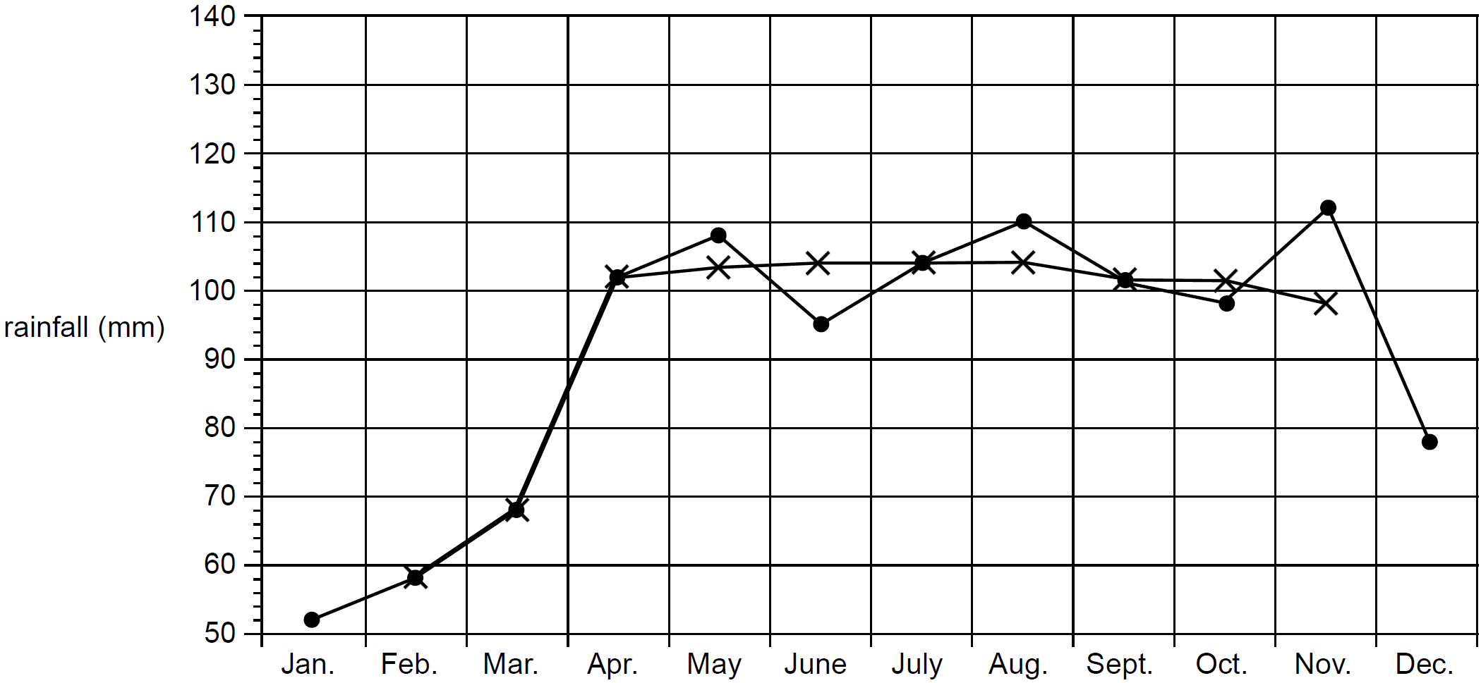
The time series plot below shows the rainfall (in mm) for each month during 2008.

- Which month had the highest rainfall? (1 mark)
--- 1 WORK AREA LINES (style=lined) ---
- Use three-median smoothing to smooth the time series. Plot the smoothed time series on the plot above.
- Mark each smoothed data point with a cross (×). (2 marks)
--- 0 WORK AREA LINES (style=lined) ---
- Describe the general pattern in rainfall that is revealed by the smoothed time series plot. (1 mark)
--- 3 WORK AREA LINES (style=lined) ---
Show Answers Only
- `text(November)`
-
- `text(Until April, the rainfall increases each month)`
`text(and then it remains relatively constant until)`
`text(November).`
Show Worked Solution
a. `text(November)`
| b. |  |
MARKER’S COMMENT: Locate medians graphically by inspection. Explaining a general pattern with more than one trend proved challenging.
c. `text(Until April, there is an increase in rainfall)`
`text(and then it remains relatively constant until)`
`text(November.)`
CORE, FUR2 2010 VCAA 3
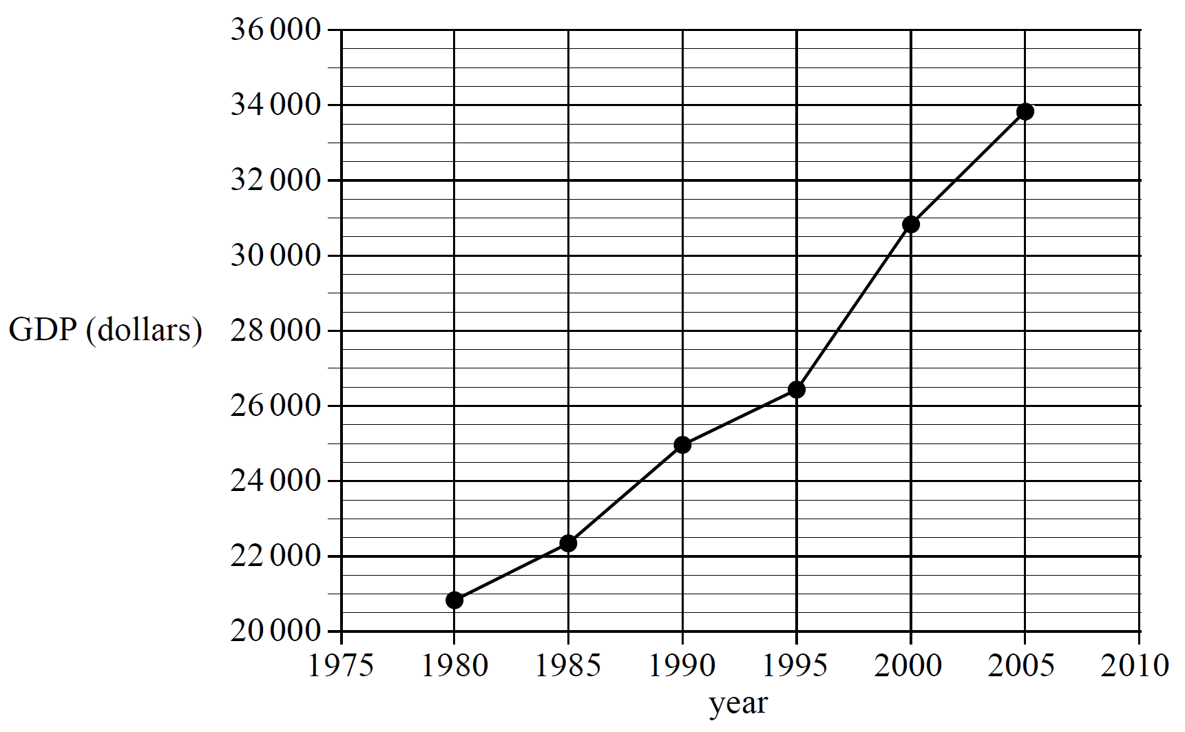
Table 2 shows the Australian gross domestic product (GDP) per person, in dollars, at five yearly intervals for the period 1980 to 2005.

- Complete the time series plot above by plotting the GDP for the years 2000 and 2005. (1 mark)
--- 0 WORK AREA LINES (style=lined) ---
- Briefly describe the general trend in the data. (1 mark)
--- 1 WORK AREA LINES (style=lined) ---
In Table 3, the variable year has been rescaled using 1980 = 0, 1985 = 5 and so on. The new variable is time.

- Use the variables time and GDP to write down the equation of the least squares regression line that can be used to predict GDP from time. Take time as the independent variable. (2 marks)
--- 4 WORK AREA LINES (style=lined) ---
- In the year 2007, the GDP was $34 900. Find the error in the prediction if the least squares regression line calculated in part c. is used to predict GDP in 2007. (2 marks)
--- 3 WORK AREA LINES (style=lined) ---
Show Answers Only
-
- `text(An increasing trend.)`
- `text(GDP = 20 000 + 524 × time)`
- `752\ text(below the actual GDP)`
Show Worked Solution
| a. |  |
b. `text(An increasing trend.)`
c. `text(By calculator,)`
MARKER’S COMMENT: Students are expected to use the variables in the diagram rather than just `x` and `y`.
`text(GDP) = 20\ 000 + 524 × text(time)`
d. `text(In 2007, time = 27,)`
`text{GDP (Predicted)}\ = 20\ 000 + 524 xx 27= 34\ 148`
`:.\ text(Error)\ = 34\ 900-34\ 148= 752\ \ text{(less than real GDP)}`
CORE, FUR2 2011 VCAA 3
The following time series plot shows the average age of women at first marriage in a particular country during the period 1915 to 1970.

- Use this plot to describe, in general terms, the way in which the average age of women at first marriage in this country has changed during the period 1915 to 1970. (1 mark)
--- 3 WORK AREA LINES (style=lined) ---
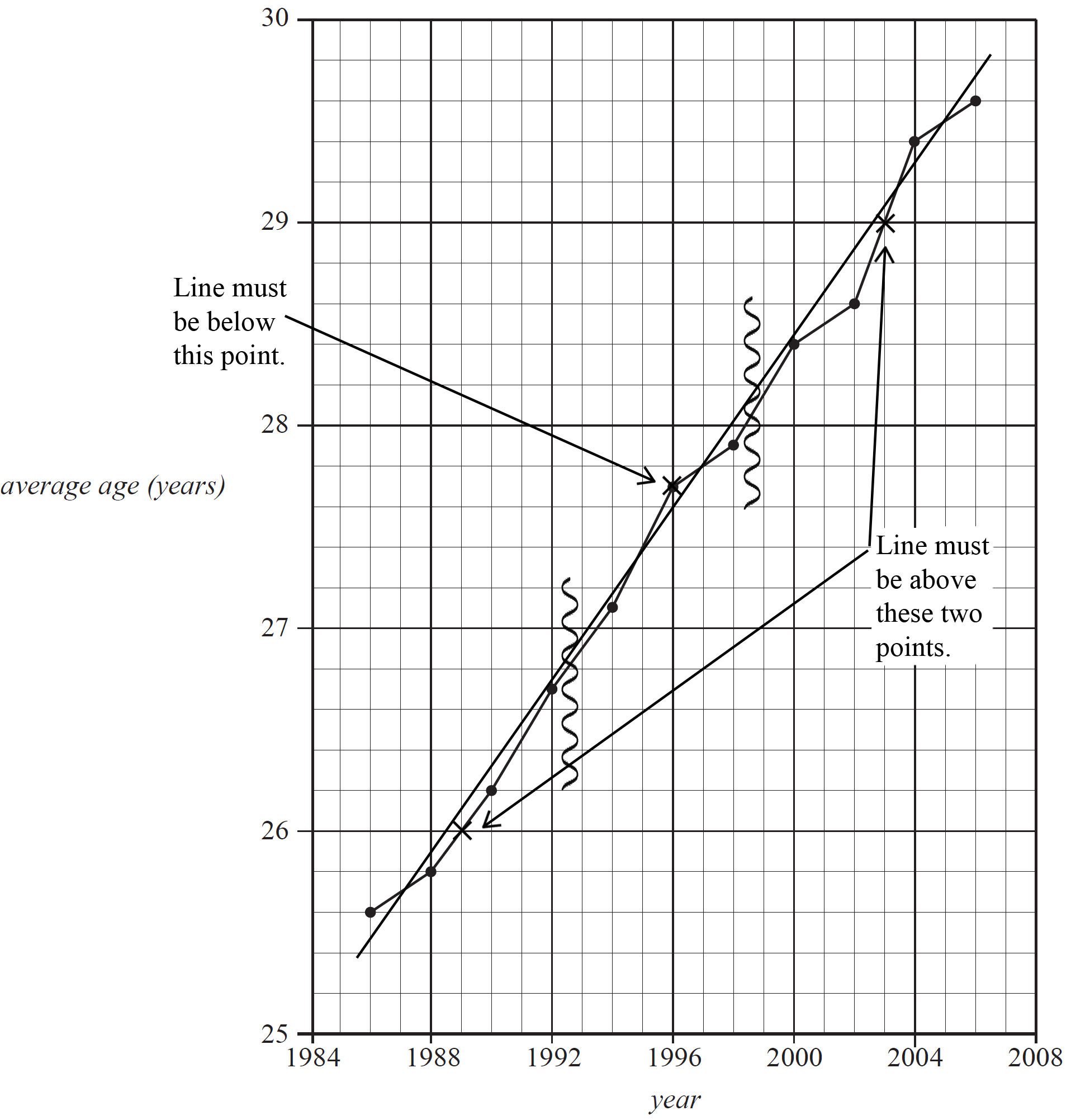
During the period 1986 to 2006, the average age of men at first marriage in a particular country indicated an increasing linear trend, as shown in the time plot below.

A three-median line could be used to model this trend.
- On the graph above
- i. clearly mark with a cross (×) the three points that would be used to fit a three-median line to this time series plot. (2 marks)
--- 0 WORK AREA LINES (style=lined) ---
- ii. draw in the three-median line. (1 mark)
--- 0 WORK AREA LINES (style=lined) ---
Show Answers Only
- `text(Constant between 1915 and 1935 and then)`
`text(decreasing between 1935 and 1970.)` -
Show Worked Solution
a. `text(The average age of women at first marriage was fairly)`
`text(constant between 1915 and 1935, and then decreased)`
`text(between 1935 and 1970.)`
b.i. & ii.

CORE, FUR1 2007 VCAA 11-13 MC
The following information relates to Parts 1, 2 and 3.
The time series plot below shows the revenue from sales (in dollars) each month made by a Queensland souvenir shop over a three-year period.

Part 1
This time series plot indicates that, over the three-year period, revenue from sales each month showed
A. no overall trend.
B. no correlation.
C. positive skew.
D. an increasing trend only.
E. an increasing trend with seasonal variation.
Part 2
A three median trend line is fitted to this data.
Its slope (in dollars per month) is closest to
A. `125`
B. `146`
C. `167`
D. `188`
E. `255`
Part 3
The revenue from sales (in dollars) each month for the first year of the three-year period is shown below.

If this information is used to determine the seasonal index for each month, the seasonal index for September will be closest to
A. `0.80`
B. `0.82`
C. `1.16`
D. `1.22`
E. `1.26`
CORE, FUR1 2008 VCAA 11-13 MC
The time series plot below shows the number of users each month of an online help service over a twelve-month period.

Part 1
The time series plot has
A. no trend.
B. no variability.
C. seasonality only.
D. an increasing trend with seasonality.
E. an increasing trend only.
Part 2
The data values used to construct the time series plot are given below.
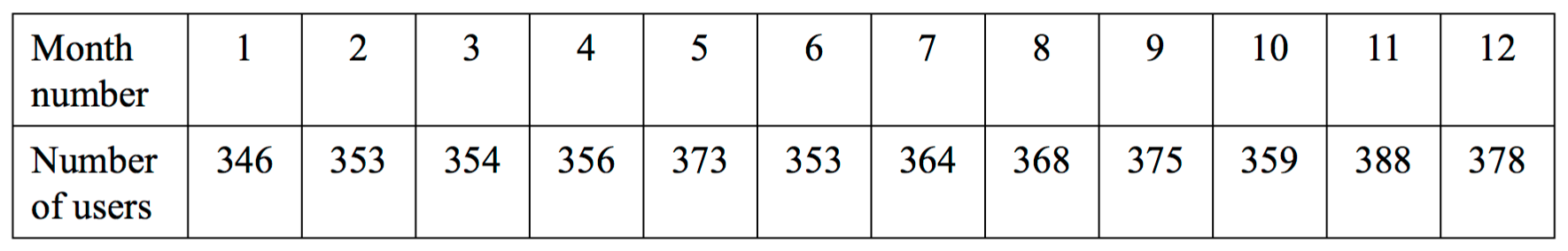
A four-point moving mean with centring is used to smooth timeline series.
The smoothed value of the number of users in month number 5 is closest to
A. `357`
B. `359`
C. `360`
D. `365`
E. `373`
Part 3
A least squares regression line is fitted to the time series plot.
The equation of this least squares regression line is
number of users = 346 + 2.77 × month number
Let month number 1 = January 2007, month number 2 = February 2007, and so on.
Using the above information, the regression line predicts that the number of users in December 2009 will be closest to
A. `379`
B. `412`
C. `443`
D. `446`
E. `448`
CORE, FUR1 2013 VCAA 12-13 MC
The time series plot below displays the number of guests staying at a holiday resort during summer, autumn, winter and spring for the years 2007 to 2012 inclusive.

Part 1
Which one of the following best describes the pattern in the time series?
A. random variation only
B. decreasing trend with seasonality
C. seasonality only
D. increasing trend only
E. increasing trend with seasonality
Part 2
The table below shows the data from the times series plot for the years 2007 and 2008.

Using four-mean smoothing with centring, the smoothed number of guests for winter 2007 is closest to
A. `85`
B. `107`
C. `183`
D. `192`
E. `200`