smc-468-30-Std Dev

Data Analysis, GEN2 2025 VCAA 1

Table 1, below, shows the prices in dollars, price, for a sample of 20 homes sold in an inner Melbourne suburb during 2017.

The type of home sold is either an apartment or a house.

Table 1

\begin{array}{|c|c|}
\hline \rule{0pt}{2.5ex}\quad \ \textit{Price(\$)}\quad \ \rule[-1ex]{0pt}{0pt}& \textit{Type} \\
\hline \rule{0pt}{2.5ex}350\,000 \rule[-1ex]{0pt}{0pt}& \ \ \text{apartment}\ \ \\
\hline \rule{0pt}{2.5ex}490\,000 \rule[-1ex]{0pt}{0pt}& \text{apartment}\\
\hline \rule{0pt}{2.5ex}500\,000 \rule[-1ex]{0pt}{0pt}& \text{apartment}\\
\hline \rule{0pt}{2.5ex}620\,000 \rule[-1ex]{0pt}{0pt}& \text{apartment}\\
\hline \rule{0pt}{2.5ex}720\,000 \rule[-1ex]{0pt}{0pt}\rule[-1ex]{0pt}{0pt}& \text{apartment}\\
\hline \rule{0pt}{2.5ex}830\,000 & \text{apartment}\\
\hline \rule{0pt}{2.5ex}875\,000 \rule[-1ex]{0pt}{0pt}& \text{apartment}\\
\hline \rule{0pt}{2.5ex}995\,000 \rule[-1ex]{0pt}{0pt}& \text{apartment}\\
\hline \rule{0pt}{2.5ex}1\,100\,000 \rule[-1ex]{0pt}{0pt}& \text{apartment}\\
\hline \rule{0pt}{2.5ex}1\,520\,000 \rule[-1ex]{0pt}{0pt}& \text{apartment}\\
\hline \rule{0pt}{2.5ex}800\,000 \rule[-1ex]{0pt}{0pt} & \text{house}\\
\hline \rule{0pt}{2.5ex}840\,000 \rule[-1ex]{0pt}{0pt}& \text{house}\\
\hline \rule{0pt}{2.5ex}920\,000 \rule[-1ex]{0pt}{0pt}& \text{house} \\
\hline \rule{0pt}{2.5ex}920\,000 \rule[-1ex]{0pt}{0pt}& \text{house}\\
\hline \rule{0pt}{2.5ex}1\,010\,000\rule[-1ex]{0pt}{0pt} & \text{house}\\
\hline \rule{0pt}{2.5ex}1\,263\,000 \rule[-1ex]{0pt}{0pt}& \text{house}\\
\hline \rule{0pt}{2.5ex}1\,398\,000 \rule[-1ex]{0pt}{0pt}& \text{house}\\
\hline \rule{0pt}{2.5ex}1\,460\,000\rule[-1ex]{0pt}{0pt} & \text{house}\\
\hline \rule{0pt}{2.5ex}1\,540\,000 \rule[-1ex]{0pt}{0pt}& \text{house} \\
\hline \rule{0pt}{2.5ex}1\,540\,000 \rule[-1ex]{0pt}{0pt} & \text{house}\\
\hline
\end{array}

Find the median, in dollars, of the variable price. (1 mark)

--- 1 WORK AREA LINES (style=lined) ---
State whether the variable type is numerical, nominal or ordinal. (1 mark)

--- 1 WORK AREA LINES (style=lined) ---
1. Complete the table below by finding the standard deviation, to the nearest whole number, for the sale price of apartments in the sample. (1 mark)
  
  --- 0 WORK AREA LINES (style=lined) ---
2. Table 2
  \begin{array}{|c|c|}
  \hline \rule{0pt}{2.5ex} \quad \ \ \textbf{Type of home} \quad \ \ & \quad \textbf{Standard deviation of} \quad \\
  & \rule[-1ex]{0pt}{0pt}\textbf{sale price (\$)}\\
  \hline \rule{0pt}{2.5ex}\text{house} \rule[-1ex]{0pt}{0pt}& 300\,911 \\
  \hline \rule{0pt}{2.5ex}\text{apartment} \rule[-1ex]{0pt}{0pt}& \\
  \hline
  \end{array}
3. Using the information in Table 2, comment on the relative spread in the distribution of the sale prices of houses compared with apartments in this sample. (1 mark)
  
  --- 3 WORK AREA LINES (style=lined) ---
Table 3, below, shows the percentage of houses and apartments with prices in the given ranges. Some information is missing.
Use the data from Table 1 to complete Table 3.
--- 0 WORK AREA LINES (style=lined) ---
Table 3

Show Answers Only

a. $\text{Median}=920\,000$

b. $\text{Variable is nominal}$

c.i. $\text{Std deviation = \$346 466}$

c.ii. $\text {Apartment sale prices have a higher spread (standard deviation) than the}$

$\text{spread of house sale prices.}$

\begin{array}{|c|c|}
\hline \hline \rule{0pt}{2.5ex}\ \ \ \text {House}(\%) \ \ \ \rule[-1ex]{0pt}{0pt}& \text {Apartment}(\%) \\
\hline \hline \rule{0pt}{2.5ex}0 \rule[-1ex]{0pt}{0pt}& 30 \\
\hline \hline \rule{0pt}{2.5ex}40 \rule[-1ex]{0pt}{0pt}& 50 \\
\hline \hline \rule{0pt}{2.5ex}60 \rule[-1ex]{0pt}{0pt}& 20 \\
\hline \hline \rule{0pt}{2.5ex}100 \rule[-1ex]{0pt}{0pt}& 100 \\
\hline
\end{array}

Show Worked Solution

a. $\text{Median}=\dfrac{10^{\text{th}}+11^{\text{th}}}{2}=920\,000$

b. $\text{Type is qualitative and cannot be ordered}$

$\Rightarrow \ \text{Variable is nominal}$

c.i. $\text{By calculator,}$

$\text{Std deviation = \$346 466}$

c.ii. $\text {Apartment sale prices have a higher spread (standard deviation) than the}$

$\text{spread of house sale prices.}$

♦ Mean mark (c.ii) 47%.

Data Analysis, GEN2 2024 NHT 1

Data was collected to investigate the behaviour of tides in Sydney Harbour.

There are usually two high tides and two low tides each day.

The variables in this study were:

Day: the day number in the sample
LLT: the height of the lowest low tide for that day (in metres)
HHT: the height of the highest high tide for that day (in metres)

Table 1 displays the data collected for a sample of 14 consecutive days in February 2021.

Table 1

\begin{array}{|c|c|c|}
\hline
\rule{0pt}{2.5ex}\ \ \ \textit{Day}\ \ \ \rule[-1ex]{0pt}{0pt}& \textit{LLT (m)} & \textit{HHT (m)}\\
\hline \rule{0pt}{2.5ex}1 \rule[-1ex]{0pt}{0pt}& 0.43 & 1.65 \\
\hline \rule{0pt}{2.5ex}2 \rule[-1ex]{0pt}{0pt}& 0.49 & 1.55 \\
\hline \rule{0pt}{2.5ex}3 \rule[-1ex]{0pt}{0pt}& 0.55 & 1.44 \\
\hline \rule{0pt}{2.5ex}4 \rule[-1ex]{0pt}{0pt}& 0.61 & 1.42 \\
\hline \rule{0pt}{2.5ex}5 \rule[-1ex]{0pt}{0pt}& 0.68 & 1.42 \\
\hline \rule{0pt}{2.5ex}6 \rule[-1ex]{0pt}{0pt}& 0.73 & 1.42 \\
\hline \rule{0pt}{2.5ex}7 \rule[-1ex]{0pt}{0pt}& 0.72 & 1.42 \\
\hline \rule{0pt}{2.5ex}8 \rule[-1ex]{0pt}{0pt}& 0.65 & 1.47 \\
\hline \rule{0pt}{2.5ex}9 \rule[-1ex]{0pt}{0pt}& 0.57 & 1.55 \\
\hline \rule{0pt}{2.5ex}10 \rule[-1ex]{0pt}{0pt}& 0.48 & 1.64 \\
\hline \rule{0pt}{2.5ex}11 \rule[-1ex]{0pt}{0pt}& 0.39 & 1.74 \\
\hline \rule{0pt}{2.5ex}12 \rule[-1ex]{0pt}{0pt}& 0.30 & 1.83 \\
\hline \rule{0pt}{2.5ex}13 \rule[-1ex]{0pt}{0pt}& 0.25 & 1.90 \\
\hline \rule{0pt}{2.5ex}14 \rule[-1ex]{0pt}{0pt}& 0.22 & 1.92 \\
\hline
\end{array}

For the $H H T$ values in Table 1:
1. Calculate the mean, in metres.
2. Round your answer to one decimal place. (1 mark)
  
  --- 2 WORK AREA LINES (style=lined) ---
3. Calculate the standard deviation, in metres.
4. Round your answer to three decimal places. (1 mark)
  
  --- 2 WORK AREA LINES (style=lined) ---
Use the $HHT$ data from Table 1 to construct a boxplot on the grid below. (2 marks)

--- 0 WORK AREA LINES (style=lined) ---

The five-number summary of the $L L T$ data is shown in Table 2 below.
Table 2

\begin{array}{|c|c|c|c|c|}
\hline \rule{0pt}{2.5ex}\textbf{Minimum} \rule[-1ex]{0pt}{0pt}& \ \ \textbf{Q1} \ \ & \textbf{Median} & \ \ \textbf{Q3} \ \ & \textbf{Maximum} \\
\hline \rule{0pt}{2.5ex}0.22 \rule[-1ex]{0pt}{0pt}& 0.39 & 0.52 & 0.65 & 0.73 \\
\hline
\end{array}

Show that the minimum $L L T$ value of 0.22 m is not an outlier. (2 marks)

--- 4 WORK AREA LINES (style=lined) ---
A least squares line can be used to model the association between $L L T$ and $H H T$. In this model, $H H T$ is the response variable.
Use the data from Table 1 to determine the equation of this least squares line.
Round the values of the intercept and slope to four significant figures.
Write your answers in the boxes provided. (2 marks)

--- 0 WORK AREA LINES (style=lined) ---

Show Answers Only

a.i. $\text{Mean = 1.6}$

a.ii. $\text{Std dev = 0.185}$

c. $IQR (LLT) = 0.65-0.39=0.26$

$\text{Lower fence}\ =Q_1-1.5 \times IQR = 0.39-1.5 \times o.26=0$

$\text{Since 0.22 > 0, 0.22 is not an outlier.}$

d. $HHT = 2.130 + (-1.054) \times LLT$

Show Worked Solution

a.i. $\text{Mean = 1.6}$

a.ii. $\text{Std dev = 0.185}$

b. $\text{Order \(HHT$ data:}\)

$1.42, 1.42, 1.42, [1.42], 1,44, 1.47, 1.55 | 1.55, 1.64, 1.65, [1.74],$

$1.83, 1.90, 1.92$

$\text{High = 1.92, Low = 1.42, \(Q_1=1.42, Q_3=1.74$, Median = 1.55}\)

c. $IQR (LLT) = 0.65-0.39=0.26$

$\text{Lower fence}\ =Q_1-1.5 \times IQR = 0.39-1.5 \times 0.26=0$

$\text{Since 0.22 > 0, 0.22 is not an outlier.}$

d. $HHT\ \text{is the response \((y)$ variable.}\)

$\text{By CAS:}$

$HHT = 2.130 + (-1.054) \times LLT$

Data Analysis, GEN1 2024 NHT 3 MC

The dot plot below displays the number of errors made in a test, for a sample of 15 students.

The mean and standard deviation for the number of errors are closest to

mean $=2.60 \quad$ standard deviation $=7.47$
mean $=2.70 \quad$ standard deviation $=7.47$
mean $=8.00 \quad$ standard deviation $=3.00$
mean $=7.47 \quad$ standard deviation $=2.60$
mean $=7.47 \quad$ standard deviation $=2.70$

Show Answers Only

$E$

Show Worked Solution

$\text{Using CAS (input dataset):}$

$3,3,4,5,6,7,8,8,8,9,10,10,10,10,11$

$\text{Mean = 7.47,}\ \ \sigma =2.70$

$\Rightarrow E$

Data Analysis, GEN1 2022 VCAA 4 MC

The age, in years, of a sample of 14 possums is displayed in the dot plot below.

The mean and the standard deviation of age for this sample of possums are closest to

mean = 4.25 standard deviation = 2.6
mean = 4.8 standard deviation = 2.4
mean = 4.8 standard deviation = 2.5
mean = 4.9 standard deviation = 2.4
mean = 4.9 standard deviation = 2.5

Show Answers Only

$E$

Show Worked Solution

$\text{By calculator:}$

$\text{Sample standard deviation} = 2.525…$

$\text{Mean} = 4.928…$

$\Rightarrow E$

Data Analysis, GEN2 2019 NHT 1

The table below displays the average sleep time, in hours, for a sample of 19 types of mammals.

Which of the two variables, type of mammal or average sleep time, is a nominal variable? (1 mark)

--- 1 WORK AREA LINES (style=lined) ---
Determine the mean and standard deviation of the variable average sleep time for this sample of mammals.
Round your answer to one decimal place. (1 mark)

--- 2 WORK AREA LINES (style=lined) ---
The average sleep time for a human is eight hours.
What percentage of this sample of mammals has an average sleep time that is less than the average sleep time for a human.
Round your answer to one decimal place. (1 mark)

--- 2 WORK AREA LINES (style=lined) ---
The sample is increase in size by adding in the average sleep time of the little brown bat.
Its average sleep time is 19.9 hours.
By how many many hours will the range for average sleep time increase when the average sleep time for the little brown bat is added to the sample? (1 mark)

--- 2 WORK AREA LINES (style=lined) ---

Show Answers Only

`text(type of mammal)`
`text(mean)= 9.2 \ text(hours)`

`sigma = 4.2 \ text(hours)`
`31.6text(%)`
`5.4 \ text(hours)`

Show Worked Solution

a. `text(type of mammal is nominal)`

b. `text(mean)= 9.2 \ text(hours) \ \ text{(by CAS)}`

`sigma = 4.2 \ text(hours) \ \ text{(by CAS)}`

c. `text(Percentage)`	`= (6)/(19) xx 100`
	`= 0.3157 …`
	`= 31.6text(%)`

d. `text(Range increase)`	`= 19.9-14.5`
	`= 5.4 \ text(hours)`

CORE, FUR1 2015 VCAA 3 MC

The dot plot below displays the difference between female and male life expectancy, in years, for a sample of 20 countries.

The mean (`barx`) and standard deviation (`s`) for this data are

A. `text(mean)\ = 2.32`	`\ \ \ \ \ text(standard deviation)\ = 5.25`
B. `text(mean)\ = 2.38`	`\ \ \ \ \ text(standard deviation)\ = 5.25`
C. `text(mean)\ = 5.0`	`\ \ \ \ \ text(standard deviation)\ = 2.0`
D. `text(mean)\ = 5.25`	`\ \ \ \ \ text(standard deviation)\ = 2.32`
E. `text(mean)\ = 5.25`	`\ \ \ \ \ text(standard deviation)\ = 2.38`

Show Answers Only

`E`

Show Worked Solution

`text(By calculator.)`

`=> E`

CORE, FUR1 2011 VCAA 6-8 MC

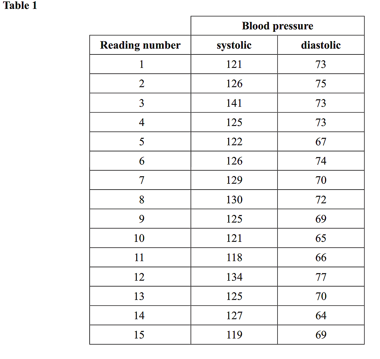
When blood pressure is measured, both the systolic (or maximum) pressure and the diastolic (or minimum) pressure are recorded.

Table 1 displays the blood pressure readings, in mmHg, that result from fifteen successive measurements of the same person's blood pressure.

Part 1

Correct to one decimal place, the mean and standard deviation of this person's systolic blood pressure measurements are respectively

A. `124.9 and 4.4`

B. `125.0 and 5.8`

C. `125.0 and 6.0`

D. `125.9 and 5.8`

E. `125.9 and 6.0`

Part 2

Using systolic blood pressure (systolic) as the response variable, and diastolic blood pressure (diastolic) as the explanatory variable, a least squares regression line is fitted to the data in Table 1.

The equation of the least squares regression line is closest to

A. `text(systolic) = 70.3 + 0.790 xx text(diastolic)`

B. `text(diastolic) = 70.3 + 0.790 xx text(systolic)`

C. `text(systolic) = 29.3 + 0.330 xx text(diastolic)`

D. `text(diastolic) = 0.330 + 29.3 xx text(systolic)`

E. `text(systolic) = 0.790 + 70.3 xx text(diastolic)`

Part 3

From the fifteen blood pressure measurements for this person, it can be concluded that the percentage of the variation in systolic blood pressure that is explained by the variation in diastolic blood pressure is closest to

A. `25.8text(%)`

B. `50.8text(%)`

C. `55.4text(%)`

D. `71.9text(%)`

E. `79.0text(%)`

Show Answers Only

`text(Part 1:)\ E`

`text(Part 2:)\ A`

`text(Part 3:)\ A`

Show Worked Solution

`text(Part 1)`

`text{By calculator (using sample standard deviation)}`

`text{the results are: }`

`text(Mean = 125.9, std dev = 6.0)`

`=>E`

`text(Part 2)`

`text{By calculator (making sure diastolic values are}`

`text{the explanatory or}\ x text{-variable), the regression line}`

`text(can be expressed as follows,)`

`text(systolic) = 70.3 + 0.790 xx text(diastolic)`

`=>A`

`text(Part 3)`

`text{By calculator, the regression line (above) should}`

`text(have found) \ \ r^2 = 0.258,\ text(which means that)`

`text(25.8% of the variation in systolic pressure can be)`

`text(explained by variation in diastolic pressure.)`

`=>A`

CORE, FUR1 2008 VCAA 5 MC

A sample of 14 people were asked to indicate the time (in hours) they had spent watching television on the previous night. The results are displayed in the dot plot below.

Correct to one decimal place, the mean and standard deviation of these times are respectively

A. `bar x=2.0\ \ \ \ \ s=1.5`

B. `bar x=2.1\ \ \ \ \ s=1.5`

C. `bar x=2.1\ \ \ \ \ s=1.6`

D. `bar x=2.6\ \ \ \ \ s=1.2`

E. `bar x=2.6\ \ \ \ \ s=1.3`

Show Answers Only

`C`

Show Worked Solution

`text(Data points are:)`

`0,0,0,1,1,2,2,2,2,3,3,4,4,5`

`text(By calculator (using sample standard deviation))`

`bar x=2.1,\ \ s=1.6`

`=> C`

CORE, FUR1 2014 VCAA 3-5 MC

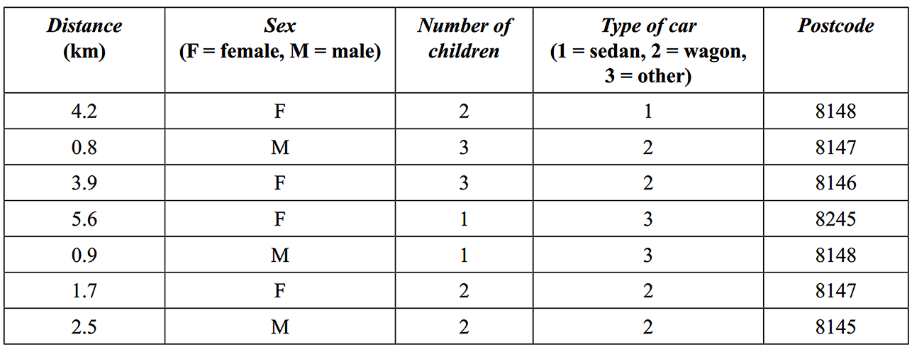
The following table shows the data collected from a sample of seven drivers who entered a supermarket car park. The variables in the table are:

distance – the distance that each driver travelled to the supermarket from their home

- sex – the sex of the driver (female, male)
- number of children – the number of children in the car
- type of car – the type of car (sedan, wagon, other)
- postcode – the postcode of the driver’s home.

Part 1

The mean, `barx`, and the standard deviation, `s_x`, of the variable, distance, are closest to

A. `barx = 2.5\ \ \ \ \ \ \s_x = 3.3`

B. `barx = 2.8\ \ \ \ \ \ \s_x = 1.7`

C. `barx = 2.8\ \ \ \ \ \ \s_x = 1.8`

D. `barx = 2.9\ \ \ \ \ \ \s_x = 1.7`

E. `barx = 3.3\ \ \ \ \ \ \s_x = 2.5`

Part 2

The number of categorical variables in this data set is

A. `0`

B. `1`

C. `2`

D. `3`

E. `4`

Part 3

The number of female drivers with three children in the car is

A. `0`

B. `1`

C. `2`

D. `3`

E. `4`

Show Answers Only

`text(Part 1:) \ C`

`text(Part 2:)\ D`

`text(Part 3:)\ B`

Show Worked Solution

`text(Part 1)`

`text(By calculator)`

`text(Distance)\ \ barx`	`=2.8`
`s_x`	`≈1.822`

`=>C`

`text(Part 2)`

♦♦ Mean mark 29%.
MARKER’S NOTE: Postcodes here are categorical variables. Ask yourself “Does it make sense to calculate the mean of this variable?” If the answer is “No”, the variable is categorical.

`text(Categorical variables are sex, type)`

`text(of car, and post code.)`

`=>D`

`text(Part 3)`

`text(1 female driver has 3 children.)`

`=>B`