The Olympic gold medal-winning height for the women's high jump, \(\textit{Wgold}\), is often lower than the best height achieved in other international women's high jump competitions in that same year. The table below lists the Olympic year, \(\textit{year}\), the gold medal-winning height, \(\textit{Wgold}\), in metres, and the best height achieved in all international women's high jump competitions in that same year, \(\textit{Wbest}\), in metres, for each Olympic year from 1972 to 2020. A scatterplot of \(\textit{Wbest}\) versus \(\textit{Wgold}\) for this data is also provided. When a least squares line is fitted to the scatterplot, the equation is found to be: \(Wbest =0.300+0.860 \times Wgold\) The correlation coefficient is 0.9318 --- 1 WORK AREA LINES (style=lined) --- --- 0 WORK AREA LINES (style=lined) --- --- 1 WORK AREA LINES (style=lined) --- --- 0 WORK AREA LINES (style=lined) --- \begin{array}{|l|l|} --- 3 WORK AREA LINES (style=lined) --- --- 4 WORK AREA LINES (style=lined) --- --- 0 WORK AREA LINES (style=lined) --- --- 3 WORK AREA LINES (style=lined) --- --- 2 WORK AREA LINES (style=lined) --- a. \(Wbest\) b. c. \(86.8\%\) d. \(\text{Strong, positive}\) e. \(Wbest\ \text{will increase, on average, by 0.86 metres for every metre of increase in}\ Wgold.\) \(\therefore\ \text{Residual}\ =2.07-2.0372=0.0328\) g.i. g.ii. \(\text{Yes, it is justified as there is no clear pattern, linear or otherwise.}\) h. \(\text{This prediction is outside the data range (1972 – 2020 → extrapolation)}\) \(\text{and therefore cannot be relied upon.}\) a. \(Wbest\) b. \(\text{Using points:}\ (1.90, 1.934)\ \text{and}\ (2.00, 2.02)\) c. \(r=0.9318\ \ \Rightarrow\ \ r^2=0.9318^2=0.8682\dots\) \(\therefore\ \text{Coefficient of determination} \approx 86.8\%\) d. \(\text{Strong, positive}\) e. \(Wbest\ \text{will increase, on average, by 0.86 metres for every metre of increase in}\ Wgold.\) g.i. g.ii. \(\text{Yes, it is justified as there is no clear pattern, linear or otherwise.}\)
h. \(\text{This prediction is outside the data range (1972–2020 → extrapolation)}\) \(\text{and therefore cannot be relied upon.}\)


\hline
\rule{0pt}{2.5ex}\text { strength } \rule[-1ex]{0pt}{0pt} & \quad \quad\quad\quad\quad\quad\quad\quad\quad\quad\quad\\
\hline
\rule{0pt}{2.5ex}\text { direction } \rule[-1ex]{0pt}{0pt} & \\
\hline
\end{array}


f.
\(Wbest\)
\(=0.300 +0.86\times 2.02\)
\(=2.0372\)

f.
\(Wbest\)
\(=0.300 +0.86\times 2.02\)
\(=2.0372\)
\(\therefore\ \text{Residual}\ =2.07-2.0372=0.0328\)
♦ Mean mark (g)(ii) 40%.
Data Analysis, GEN2 2024 VCAA 1
Table 1 lists the Olympic year, \(\textit{year}\), and the gold medal-winning height for the men's high jump, \(\textit{Mgold}\), in metres, for each Olympic Games held from 1928 to 2020. No Olympic Games were held in 1940 or 1944, and the 2020 Olympic Games were held in 2021. Table 1 \begin{array}{|c|c|} --- 1 WORK AREA LINES (style=lined) --- --- 2 WORK AREA LINES (style=lined) --- --- 3 WORK AREA LINES (style=lined) --- --- 0 WORK AREA LINES (style=lined) --- --- 0 WORK AREA LINES (style=lined) --- --- 4 WORK AREA LINES (style=lined) --- a.i. \(2.39\) a.ii. \(50\%\) b. \(0.8\) c. d. e. \(\text{A coefficient of determination of 85.7% shows the variation in}\) \(\text{the}\ Mgold\ \text{that is explained by the variation in the }year.\) a.i. \(2.39\) a.ii. \(\dfrac{11}{22}=50\%\) \(Q_1=2.12, \ Q_3=2.36\) \(\text{Min}\ =1.94, \ \text{Max}\ =2.39\) e. \(\text{A coefficient of determination of 85.7% shows the variation in}\) \(\text{the}\ Mgold\ \text{that is explained by the variation in the }year.\)
\hline \quad \textit{year} \quad & \textit{Mgold}\,\text{(m)} \\
\hline 1928 & 1.94 \\
\hline 1932 & 1.97 \\
\hline 1936 & 2.03 \\
\hline 1948 & 1.98 \\
\hline 1952 & 2.04 \\
\hline 1956 & 2.12 \\
\hline 1960 & 2.16 \\
\hline 1964 & 2.18 \\
\hline 1968 & 2.24 \\
\hline 1972 & 2.23 \\
\hline 1976 & 2.25 \\
\hline 1980 & 2.36 \\
\hline 1984 & 2.35 \\
\hline 1988 & 2.38 \\
\hline 1992 & 2.34 \\
\hline 1996 & 2.39 \\
\hline 2000 & 2.35 \\
\hline 2004 & 2.36 \\
\hline 2008 & 2.36 \\
\hline 2012 & 2.33 \\
\hline 2016 & 2.38 \\
\hline 2020 & 2.37 \\
\hline
\end{array}

![]()
Show Answers Only

![]() Show Worked Solution
Show Worked Solution
b.
\(z\)
\(=\dfrac{x-\overline x}{s_x}\)
\(=\dfrac{2.35-2.23}{0.15}\)
\(=0.8\)
c. \(Q_2=\dfrac{2.33+2.25}{2}=2.29\)

Data Analysis, GEN2 2023 VCAA 1
Data was collected to investigate the use of electronic images to automate the sizing of oysters for sale. The variables in this study were: The data collected for a sample of 15 oysters is displayed in the table. --- 1 WORK AREA LINES (style=lined) --- --- 1 WORK AREA LINES (style=lined) --- --- 1 WORK AREA LINES (style=lined) --- --- 1 WORK AREA LINES (style=lined) --- --- 0 WORK AREA LINES (style=lined) --- --- 4 WORK AREA LINES (style=lined) --- --- 4 WORK AREA LINES (style=lined) ---

the median weight of the large oysters in this sample. (1 mark)
Complete the following sentence by filling in the blank space provided. (1 mark)
This equation predicts that, on average, each 10 g increase in the weight of an oyster is associated with a ________________ cm³ increase in its volume.
Data Analysis, GEN1 2023 VCAA 10 MC
A study of Year 10 students shows that there is a negative association between the scores of topic tests and the time spent on social media. The coefficient of determination is 0.72
From this information it can be concluded that
- a decreased time spent on social media is associated with an increased topic test score.
- less time spent on social media causes an increase in topic test performance.
- an increased time spent on social media is associated with an increased topic test score.
- too much time spent on social media causes a reduction in topic test performance.
- a decreased time spent on social media is associated with a decreased topic test score.
CORE, FUR2 2021 VCAA 3
The time series plot below shows the winning time, in seconds, for the women's 100 m freestyle swim plotted against year, for each year that the Olympic Games were held during the period 1956 to 2016.
A least squares line has been fitted to the plot to model the decreasing trend in the winning time over this period.

The equation of the least squares line is
winning time = 357.1 – 0.1515 × year
The coefficient of determination is 0.8794
- Name the explanatory variable in this time series plot. (1 mark)
--- 1 WORK AREA LINES (style=lined) ---
- Determine the value of the correlation coefficient (`r`).
- Round your answer to three decimal places. (1 mark)
--- 2 WORK AREA LINES (style=lined) ---
- Write down the average decrease in winning time, in seconds per year, during the period 1956 to 2016. (1 mark)
--- 2 WORK AREA LINES (style=lined) ---
- The predicted winning time for the women's 100 m freestyle in 2000 was 54.10 seconds.
- The actual winning time for the women's 100 m freestyle in 2000 was 53.83 seconds.
- Determine the residual value in seconds. (1 mark)
--- 2 WORK AREA LINES (style=lined) ---
- The following equation can be used to predict the winning time for the women's 100 m freestyle in the future.
- winning time = 357.1 – 0.1515 × year
- i. Show that the predicted winning time for the women's 100 m freestyle in 2032 is 49.252 seconds. (1 mark)
--- 2 WORK AREA LINES (style=lined) ---
- ii. What assumption is being made when this equation is used to predict the winning time for the women's 100 m freestyle in 2032? (1 mark)
--- 2 WORK AREA LINES (style=lined) ---
CORE, FUR1 2021 VCAA 11 MC
The table below shows the weight, in kilograms, and the height, in centimetres, of 10 adults.

A least squares line is fitted to the data
The least squares line enables an adult's weight to be predicted from their height.
The number of times that the predicted value of an adult's weight is greater than the actual value of their weight is
- 3
- 4
- 5
- 6
- 7
CORE, FUR2 2020 VCAA 4
The age, in years, body density, in kilograms per litre, and weight, in kilograms, of a sample of 12 men aged 23 to 25 years are shown in the table below.
| Age (years) |
Body density |
Weight |
|
| 23 | 1.07 | 70.1 | |
| 23 | 1.07 | 90.4 | |
| 23 | 1.08 | 73.2 | |
| 23 | 1.08 | 85.0 | |
| 24 | 1.03 | 84.3 | |
| 24 | 1.05 | 95.6 | |
| 24 | 1.07 | 71.7 | |
| 24 | 1.06 | 95.0 | |
| 25 | 1.07 | 80.2 | |
| 25 | 1.09 | 87.4 | |
| 25 | 1.02 | 94.9 | |
| 25 | 1.09 | 65.3 |
- For these 12 men, determine
- i. their median age, in years. (1 mark)
--- 2 WORK AREA LINES (style=lined) ---
- ii. the mean of their body density, in kilograms per litre. (1 mark)
--- 2 WORK AREA LINES (style=lined) ---
- A least squares line is to be fitted to the data with the aim of predicting body density from weight.
- i. Name the explanatory variable for this least squares line. (1 mark)
--- 1 WORK AREA LINES (style=lined) ---
- ii. Determine the slope of this least squares line.
- Round your answer to three significant figures. (1 mark)
--- 1 WORK AREA LINES (style=lined) ---
- What percentage of the variation in body density can be explained by the variation in weight?
- Round your answer to the nearest percentage. (1 mark)
--- 2 WORK AREA LINES (style=lined) ---
Data Analysis, GEN2 2019 NHT 3
The life span, in years, and gestation period, in days, for 19 types of mammals are displayed in the table below.

- A least squares line that enables life span to be predicted from gestation period is fitted to this data.
- Name the explanatory variable in the equation of this least squares line. (1 mark)
--- 1 WORK AREA LINES (style=lined) ---
- Determine the equation of the least squares line in terms of the variables life span and gestation period.
- Round the numbers representing the intercept and slope to three significant figures. (2 marks)
--- 2 WORK AREA LINES (style=lined) ---
- Write the value of the correlation rounded to three decimal places. (1 mark)
--- 2 WORK AREA LINES (style=lined) ---
CORE, FUR2 2019 VCAA 4
The relative humidity (%) at 9 am and 3 pm on 14 days in November 2017 is shown in Table 3 below.

A least squares line is to be fitted to the data with the aim of predicting the relative humidity at 3 pm (humidity 3 pm) from the relative humidity at 9 am (humidity 9 am).
- Name the explanatory variable. (1 mark)
--- 1 WORK AREA LINES (style=lined) ---
- Determine the values of the intercept and the slope of this least squares line.
- Round both values to three significant figures and write them in the appropriate boxes provided. (1 mark)
--- 0 WORK AREA LINES (style=lined) ---
| humidity 3 pm = |
|
+ |
|
× humidity 9 am (1 mark) |
- Determine the value of the correlation coefficient for this data set.
- Round your answer to three decimal places. (1 mark)
--- 1 WORK AREA LINES (style=lined) ---
CORE, FUR2 2018 VCAA 2
The congestion level in a city can be recorded as the percentage increase in travel time due to traffic congestion in peak periods (compared to non-peak periods).
This is called the percentage congestion level.
The percentage congestion levels for the morning and evening peak periods for 19 large cities are plotted on the scatterplot below.

- Determine the median percentage congestion level for the morning peak period and the evening peak period.
Write your answers in the appropriate boxes provided below. (2 marks)
--- 0 WORK AREA LINES (style=lined) ---
| Median percentage congestion level for morning peak period |
%
|
| Median percentage congestion level for evening peak period |
%
|
A least squares line is to be fitted to the data with the aim of predicting evening congestion level from morning congestion level.
The equation of this line is.
evening congestion level = 8.48 + 0.922 × morning congestion level
- Name the response variable in this equation. (1 mark)
--- 1 WORK AREA LINES (style=lined) ---
- Use the equation of the least squares line to predict the evening congestion level when the morning congestion level is 60%. (1 mark)
--- 2 WORK AREA LINES (style=lined) ---
- Determine the residual value when the equation of the least squares line is used to predict the evening congestion level when the morning congestion level is 47%.
- Round your answer to one decimal place? (2 marks)
--- 4 WORK AREA LINES (style=lined) ---
- The value of the correlation coefficient `r` is 0.92
- What percentage of the variation in the evening congestion level can be explained by the variation in the morning congestion level?
- Round your answer to the nearest whole number. (1 mark)
--- 2 WORK AREA LINES (style=lined) ---
CORE, FUR1 2018 VCAA 14 MC
A least squares line is fitted to a set of bivariate data.
Another least squares line is fitted with response and explanatory variables reversed.
Which one of the following statistics will not change in value?
- the residual values
- the predicted values
- the correlation coefficient `r`
- the slope of the least squares line
- the intercept of the least squares line
CORE, FUR2 2008 VCAA 4
The arm spans (in cm) and heights (in cm) for a group of 13 boys have been measured. The results are displayed in the table below.

The aim is to find a linear equation that allows arm span to be predicted from height.
- What will be the explanatory variable in the equation? (1 mark)
--- 1 WORK AREA LINES (style=lined) ---
- Assuming a linear association, determine the equation of the least squares regression line that enables arm span to be predicted from height. Write this equation in terms of the variables arm span and height. Give the coefficients correct to two decimal places. (2 marks)
--- 2 WORK AREA LINES (style=lined) ---
- Using the equation that you have determined in part b., interpret the slope of the least squares regression line in terms of the variables height and arm span. (1 mark)
--- 2 WORK AREA LINES (style=lined) ---
CORE, FUR2 2010 VCAA 2
In the scatterplot below, average annual female income, in dollars, is plotted against average annual male income, in dollars, for 16 countries. A least squares regression line is fitted to the data. The equation of the least squares regression line for predicting female income from male income is female income = 13 000 + 0.35 × male income --- 1 WORK AREA LINES (style=lined) --- From the least squares regression line equation it can be concluded that, for these countries, on average, female income increases by `text($________)` for each $1000 increase in male income. (1 mark) --- 0 WORK AREA LINES (style=lined) --- --- 1 WORK AREA LINES (style=lined) --- Explain why. (1 mark) --- 2 WORK AREA LINES (style=lined) ---

CORE, FUR2 2014 VCAA 2
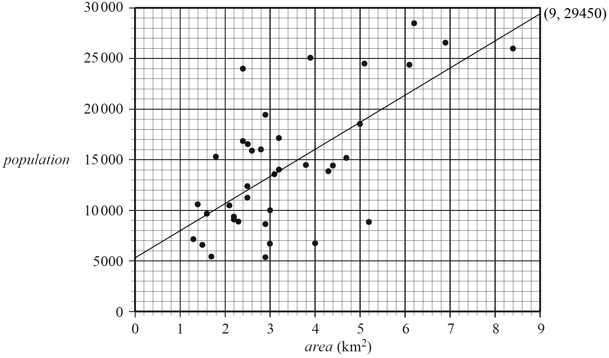
The scatterplot below shows the population and area (in square kilometres) of a sample of inner suburbs of a large city.

The equation of the least squares regression line for the data in the scatterplot is
population = 5330 + 2680 × area
- Write down the response variable. (1 mark)
--- 1 WORK AREA LINES (style=lined) ---
- Draw the least squares regression line on the scatterplot above. (1 mark)
--- 0 WORK AREA LINES (style=lined) ---
- Interpret the slope of this least squares regression line in terms of the variables area and population. (2 marks)
--- 4 WORK AREA LINES (style=lined) ---
- Wiston is an inner suburb. It has an area of 4 km² and a population of 6690.
- The correlation coefficient, `r`, is equal to 0.668
- i. Calculate the residual when the least squares regression line is used to predict the population of Wiston from its area. (1 mark)
--- 2 WORK AREA LINES (style=lined) ---
- ii. What percentage of the variation in the population of the suburbs is explained by the variaton in area.
- Write your answer, correct to one decimal place. (1 mark)
--- 2 WORK AREA LINES (style=lined) ---
Show Answers Only
- `text(Population.)`
-
- `text(Population increases by 2680 people, on average,)`
`text(for each additional 1 km² in area.)` -
- ` −9360`
- `text(44.6%)`

Show Worked Solution
a. `text(Population.)`
♦ Mean mark 36%.
MARKER’S COMMENT: Use the equation to draw the line and use points at the extremities.
MARKER’S COMMENT: Use the equation to draw the line and use points at the extremities.
| b. |
|
c. `text(Population increases by 2680 people, on average,)`
♦ Mean mark 41% (part (iii)).
`text(for each additional 1 km² in area.)`
d.i. `text(Predicted population) = 5330 + 2680 xx 4= 16\ 050`
`:.\ text(Residual)\ = 6690-16\ 050= -9360`
♦ Part (iv) in total had a mean mark 42%.
| d.ii. | `r` | `= 0.668^2` |
| `r^2` | `= 0.4462…` | |
| `= 44.6 text{% (to 1 d.p.)}` |
`:.\ text(44.6% of the variation in the population is explained)`
`text(by variation in the area.)`