Data was collected to investigate the behaviour of tides in Sydney Harbour. There are usually two high tides and two low tides each day. The variables in this study were: Table 1 displays the data collected for a sample of 14 consecutive days in February 2021. Table 1 \begin{array}{|c|c|c|} --- 2 WORK AREA LINES (style=lined) --- --- 2 WORK AREA LINES (style=lined) --- --- 0 WORK AREA LINES (style=lined) --- \begin{array}{|c|c|c|c|c|} --- 4 WORK AREA LINES (style=lined) --- --- 0 WORK AREA LINES (style=lined) --- a.i. \(\text{Mean = 1.6}\) a.ii. \(\text{Std dev = 0.185}\) b. c. \(IQR (LLT) = 0.65-0.39=0.26\) \(\text{Lower fence}\ =Q_1-1.5 \times IQR = 0.39-1.5 \times o.26=0\) \(\text{Since 0.22 > 0, 0.22 is not an outlier.}\) d. \(HHT = 2.130 + (-1.054) \times LLT\) a.i. \(\text{Mean = 1.6}\) a.ii. \(\text{Std dev = 0.185}\) b. \(\text{Order \(HHT\) data:}\) \(1.42, 1.42, 1.42, [1.42], 1,44, 1.47, 1.55 | 1.55, 1.64, 1.65, [1.74],\) \(1.83, 1.90, 1.92\) \(\text{High = 1.92, Low = 1.42, \(Q_1=1.42, Q_3=1.74\), Median = 1.55}\) \(\text{Lower fence}\ =Q_1-1.5 \times IQR = 0.39-1.5 \times 0.26=0\) \(\text{Since 0.22 > 0, 0.22 is not an outlier.}\) d. \(HHT\ \text{is the response \((y)\) variable.}\) \(\text{By CAS:}\) \(HHT = 2.130 + (-1.054) \times LLT\)
\hline
\rule{0pt}{2.5ex}\ \ \ \textit{Day}\ \ \ \rule[-1ex]{0pt}{0pt}& \textit{LLT (m)} & \textit{HHT (m)}\\
\hline \rule{0pt}{2.5ex}1 \rule[-1ex]{0pt}{0pt}& 0.43 & 1.65 \\
\hline \rule{0pt}{2.5ex}2 \rule[-1ex]{0pt}{0pt}& 0.49 & 1.55 \\
\hline \rule{0pt}{2.5ex}3 \rule[-1ex]{0pt}{0pt}& 0.55 & 1.44 \\
\hline \rule{0pt}{2.5ex}4 \rule[-1ex]{0pt}{0pt}& 0.61 & 1.42 \\
\hline \rule{0pt}{2.5ex}5 \rule[-1ex]{0pt}{0pt}& 0.68 & 1.42 \\
\hline \rule{0pt}{2.5ex}6 \rule[-1ex]{0pt}{0pt}& 0.73 & 1.42 \\
\hline \rule{0pt}{2.5ex}7 \rule[-1ex]{0pt}{0pt}& 0.72 & 1.42 \\
\hline \rule{0pt}{2.5ex}8 \rule[-1ex]{0pt}{0pt}& 0.65 & 1.47 \\
\hline \rule{0pt}{2.5ex}9 \rule[-1ex]{0pt}{0pt}& 0.57 & 1.55 \\
\hline \rule{0pt}{2.5ex}10 \rule[-1ex]{0pt}{0pt}& 0.48 & 1.64 \\
\hline \rule{0pt}{2.5ex}11 \rule[-1ex]{0pt}{0pt}& 0.39 & 1.74 \\
\hline \rule{0pt}{2.5ex}12 \rule[-1ex]{0pt}{0pt}& 0.30 & 1.83 \\
\hline \rule{0pt}{2.5ex}13 \rule[-1ex]{0pt}{0pt}& 0.25 & 1.90 \\
\hline \rule{0pt}{2.5ex}14 \rule[-1ex]{0pt}{0pt}& 0.22 & 1.92 \\
\hline
\end{array}

\hline \rule{0pt}{2.5ex}\textbf{Minimum} \rule[-1ex]{0pt}{0pt}& \ \ \textbf{Q1} \ \ & \textbf{Median} & \ \ \textbf{Q3} \ \ & \textbf{Maximum} \\
\hline \rule{0pt}{2.5ex}0.22 \rule[-1ex]{0pt}{0pt}& 0.39 & 0.52 & 0.65 & 0.73 \\
\hline
\end{array}
![]()

c. \(IQR (LLT) = 0.65-0.39=0.26\)
Data Analysis, GEN2 2019 NHT 2
The five-number summary below was determined from the sleep time, in hours, of a sample of 59 types of mammals. \begin{array} {|l|c|} --- 5 WORK AREA LINES (style=lined) --- --- 0 WORK AREA LINES (style=lined) ---
\hline
\rule{0pt}{2.5ex} \ \ \ \textbf{Statistic} \rule[-1ex]{0pt}{0pt} & \textbf{Sleep time (hours)} \\
\hline
\rule{0pt}{2.5ex} \text{minimum} \rule[-1ex]{0pt}{0pt} & \text{2.5} \\
\hline
\rule{0pt}{2.5ex} \text{first quartile} \rule[-1ex]{0pt}{0pt} & \text{8.0} \\
\hline
\rule{0pt}{2.5ex} \text{median} \rule[-1ex]{0pt}{0pt} & \text{10.5} \\
\hline
\rule{0pt}{2.5ex} \text{third quartile} \rule[-1ex]{0pt}{0pt} & \text{13.5} \\
\hline
\rule{0pt}{2.5ex} \text{maximum} \rule[-1ex]{0pt}{0pt} & \text{20.0} \\
\hline
\end{array}

Show Answers Only

a. `IQR = Q_3-Q_1 = 13.5-8.0 = 5.5` `=> \ text(no outliers)` b. Show Worked Solution
`text(Lower fence)`
`= Q_1-1.5 xx IQR`
`= 8-1.5 xx 5.5`
`= -0.25`
`text(Upper fence)`
`= Q_3 + 1.5 xx IQR`
`= 13.5 + 1.5 xx 5.5`
`= 21.75`
`text(S) text(ince) \ -0.25 < 2.5 \ text{(minimum value) and} \ 21.75 > 20.0 \ text{(maximum value)}`
CORE, FUR2 2016 VCAA 2
A weather station records daily maximum temperatures.
- The five-number summary for the distribution of maximum temperatures for the month of February is displayed in the table below.

- There are no outliers in this distribution.
- i. Use the five-number summary above to construct a boxplot on the grid below. (1 mark)
--- 0 WORK AREA LINES (style=lined) ---

- ii. What percentage of days had a maximum temperature of 21°C, or greater, in this particular February? (1 mark)
--- 2 WORK AREA LINES (style=lined) ---
- The boxplots below display the distribution of maximum daily temperature for the months of May and July.
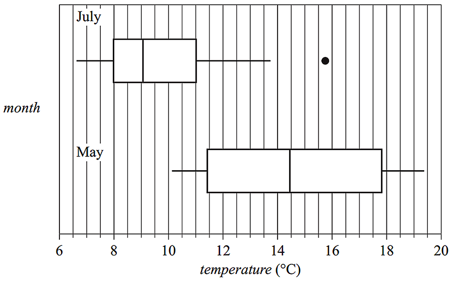
- i. Describe the shapes of the distributions of daily temperature (including outliers) for July and for May. (1 mark)
--- 2 WORK AREA LINES (style=lined) ---
- ii. Determine the value of the upper fence for the July boxplot. (1 mark)
--- 3 WORK AREA LINES (style=lined) ---
- iii. Using the information from the boxplots, explain why the maximum daily temperature is associated with the month of the year. Quote the values of appropriate statistics in your response. (1 mark)
--- 3 WORK AREA LINES (style=lined) ---

Show Answers Only
| a.i. |  |
a.ii. `text(75%)`
| b.i. | `text(July – Positively skewed with an outlier.)` |
| `text(May – Symmetrical with no outliers.)` |
b.ii. `15.5^@\text(C)`
b.iii. `text{The median temperature in May (14.5°C)}`
`text(differs from the median temperature in July)`
`text{(just over 9°C). This difference is why the}`
`text(maximum daily temperature is associated)`
`text(with the month.)`
Show Worked Solution
| a.i. | |
a.ii. `text(75%)`
MARKER’S COMMENT: Incorrect May descriptors included “evenly or normally distributed”, “bell shaped” and “symmetrically skewed.”
| b.i. | `text(July – Positively skewed with an outlier.)` |
| `text(May – Symmetrical with no outliers.)` |
| b.ii. | `text(Upper fence)` | `= Q_3 + 1.5 xx IQR` |
| `= 11 + 1.5 xx (11 – 8)` | ||
| `= 11 + 4.5` | ||
| `= 15.5^@\text(C)` |
♦♦ Mean mark (b)(iii) – 30%.
COMMENT: Refer to the difference in medians. Just quoting the numbers was not enough to gain a mark here.
COMMENT: Refer to the difference in medians. Just quoting the numbers was not enough to gain a mark here.
b.iii. `text{The median temperature in May (14.5°C)}`
`text(differs from the median temperature in July)`
`text{(just over 9°C). This difference is why the}`
`text(maximum daily temperature is associated)`
`text(with the month.)`
CORE, FUR2 2006 VCAA 1
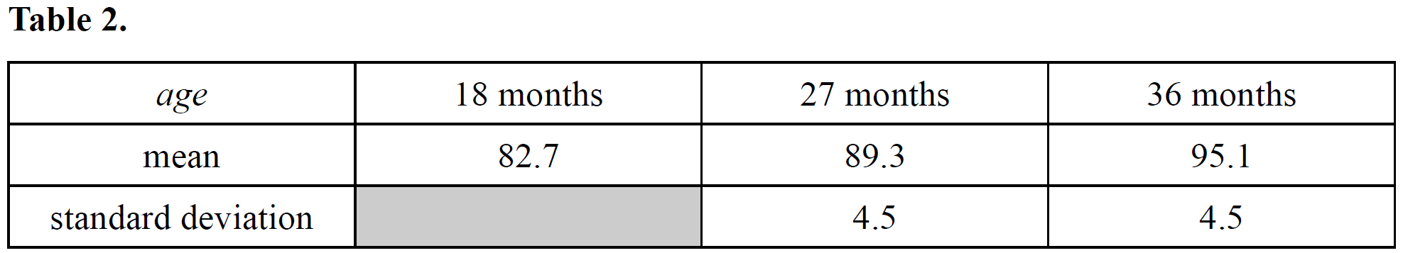
Table 1 shows the heights (in cm) of three groups of randomly chosen boys aged 18 months, 27 months and 36 months respectively.

- Complete Table 2 by calculating the standard deviation of the heights of the 18-month-old boys.
Write your answer correct to one decimal place. (1 mark)
--- 2 WORK AREA LINES (style=lined) ---

A 27-month-old boy has a height of 83.1 cm.
- Calculate his standardised height (`z` score) relative to this sample of 27-month-old boys.
- Write your answer correct to one decimal place. (1 mark)
--- 2 WORK AREA LINES (style=lined) ---
The heights of the 36-month-old boys are normally distributed.
A 36-month-old boy has a standardised height of 2.
- Approximately what percentage of 36-month-old boys will be shorter than this child? (1 mark)
--- 2 WORK AREA LINES (style=lined) ---
Using the data from Table 1, boxplots have been constructed to display the distributions of heights of 36-month-old and 27-month-old boys as shown below.

- Complete the display by constructing and drawing a boxplot that shows the distribution of heights for the 18-month-old boys. (2 marks)
--- 0 WORK AREA LINES (style=lined) ---
- Use the appropriate boxplot to determine the median height (in centimetres) of the 27-month-old boys. (1 mark)
--- 1 WORK AREA LINES (style=lined) ---
The three parallel boxplots suggest that height and age (18 months, 27 months, 36 months) are positively related.
- Explain why, giving reference to an appropriate statistic. (1 mark)
--- 1 WORK AREA LINES (style=lined) ---
Show Answers Only
- `3.8`
- `−1.4`
- `2.5 text(%)`
-
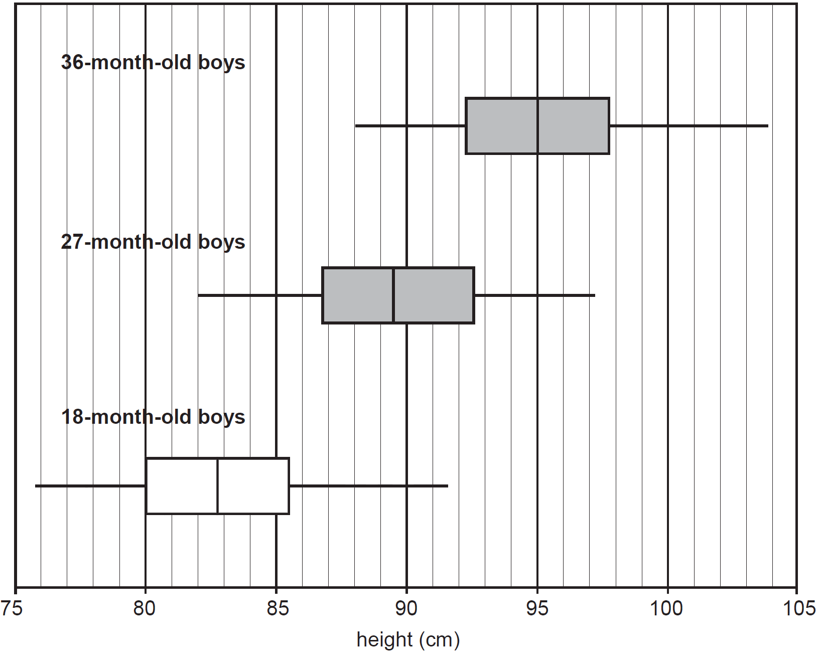
- `89.5`
- `text(Median height increases as age increases.)`
Show Worked Solution
a. `text(By calculator,)`
`text(standard deviation) = 3.8`
| b. | `z` | `= (x – barx)/s` |
| `= (83.1 – 89.3)/(4.5)` | ||
| `=-1.377…` | ||
| `= -1.4\ \ text{(1 d.p.)}` |
♦♦ MARKER’S COMMENT: Attention required here as this standard question was “very poorly answered”.
c. `text{2.5% (see graph below)}`

d. `text(Range = 76 – 89.8,)\ Q_1 = 80,\ Q_3 = 85.8,\ text(Median = 83,)`

e. `89.5`
MARKER’S COMMENT: A boxplot statistic was required, so mean values were not relevant.
f. `text(The median height increases with age.)`