The stem plot below displays 30 temperatures recorded at a weather station.

The modal temperature is
- 2.8°C
- 2.9°C
- 3.7°C
- 8.0°C
- 9.0°C
Aussie Maths & Science Teachers: Save your time with SmarterEd
The stem plot below displays 30 temperatures recorded at a weather station.
The modal temperature is
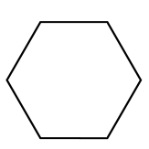
The blood pressure (low, normal, high) and the age (under 50 years, 50 years or over) of 110 adults were recorded. The results are displayed in the two-way frequency table below.
Part 1
The percentage of adults under 50 years of age who have high blood pressure is closest to
Part 2
The variables blood pressure (low, normal, high) and age (under 50 years, 50 years or over) are
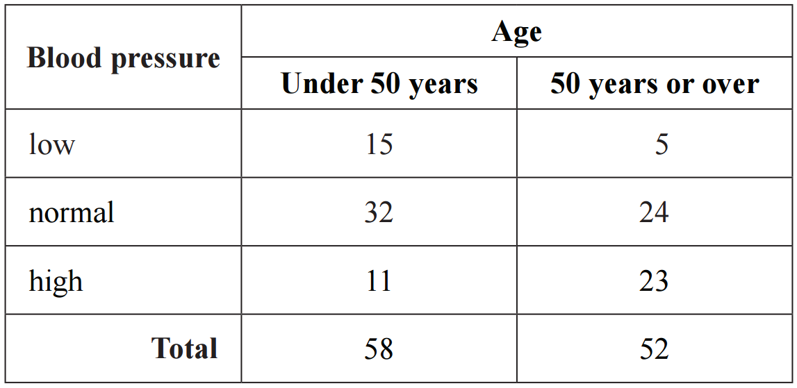
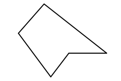
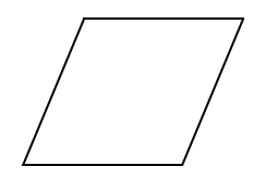
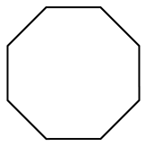
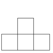
Which shape is a hexagon?
 |
 |
 |
 |
|
|
|
|
|
`text(A hexagon has 6 sides.)`

The amount of drink in this jug is
|
|
one and a half litres |
|
|
two litres |
|
|
two and a half litres |
|
|
three litres |
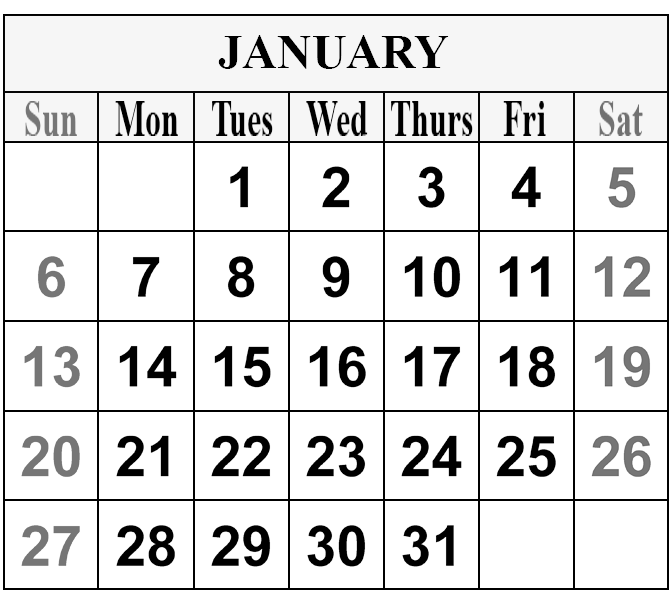
What date is the third Monday on this calendar?
| `text(28 January)` | `text(21 January)` | `text(14 January)` | `text(7 January)` |
|
|
|
|
|
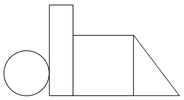
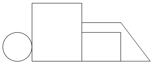
Sven made this model using blocks.
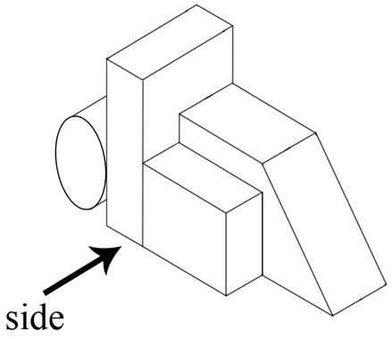
Which of these shows the view from the side?
 |
 |
|
|
|
 |
 |
|
|
|
The best description of this 3D object is a
|
|
`text(cube)` |
|
|
`text(prism)` |
|
|
`text(cylinder)` |
|
|
`text(square pyramid)` |
| `26 + 47 =` |
Each domino has 8 dots.
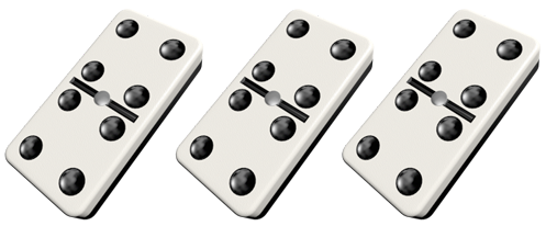
Which of these shows one way to work out the total number of dots?
| `4 + 4 + 4` | `8 + 3` | `8 - 3` | `8 + 8 + 8` |
|
|
|
|
|
The minute hand is missing.

What time could this clock be showing?
| `text(8 o'clock)` | `text(half past 8)` | `text(9 o'clock)` | `text(half past 9)` |
|
|
|
|
|
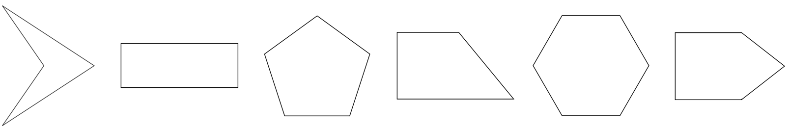
How many of these shapes have exactly 4 sides?
| `2` | `3` | `4` | `5` |
|
|
|
|
|
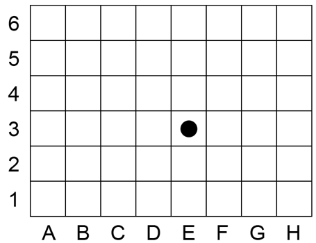
Peter moves the marker left 3 squares and then up 2 squares.
What cell does Peter move the marker to?
| `text(B1)` | `text(C6)` | `text(H5)` | `text(B5)` |
|
|
|
|
|
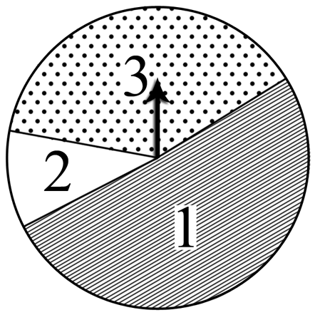
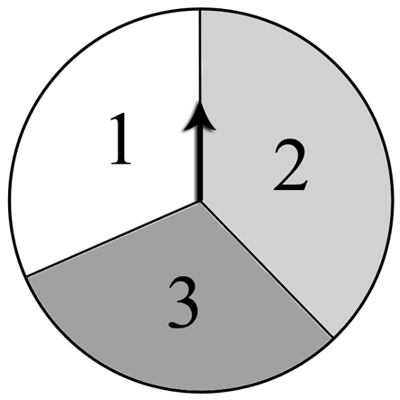
Which spinner is most likely to stop on the number 2?
 |
 |
 |
 |
|
|
|
|
|
`text(This spinner has)\ 1/2\ text(chance of landing on 2.)`
`text{(all others spinners have less chance).}`
Jesse had these shells.
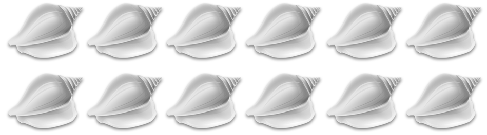
He kept 7 and gave the rest to James.
How many shells did Jesse give to James?
| `5` | `6` | `7` | `12` |
|
|
|
|
|
Children at a Summer Camp are split into four colour teams, red, yellow, blue and green.
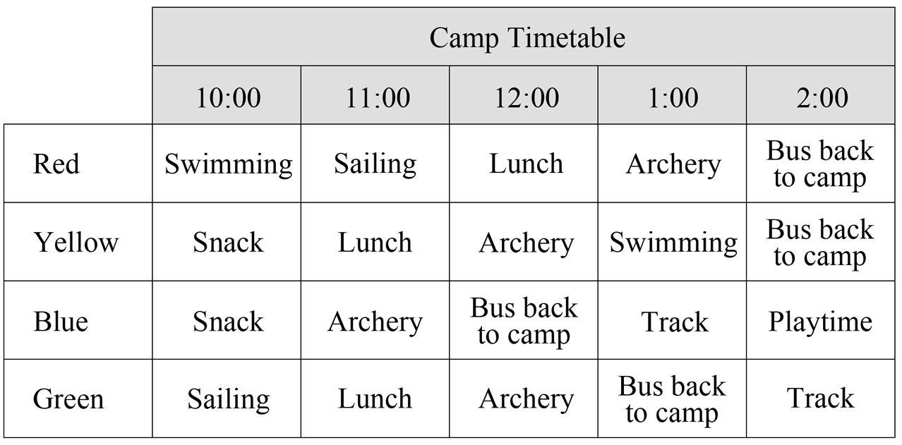
Which team has archery lessons first?
| `text(Red)` | `text(Yellow)` | `text(Blue)` | `text(Green)` |
|
|
|
|
|
Melinda placed some shells in rows of 8.

She then put the same number of shells into bags of 6 and had some left over.
How many shells were left over?
| `4` | `3` | `2` | `1` |
|
|
|
|
|
Kelly has sorted a number of shapes into groups.
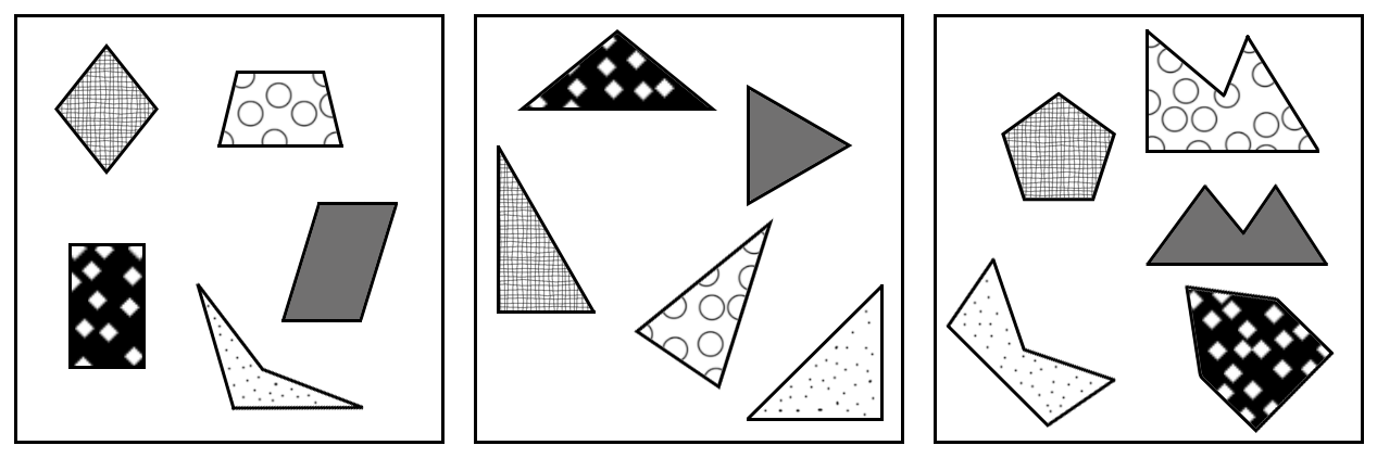
How did Kelly sort her shapes?
|
|
`text(by length of sides)` |
|
|
`text(by type of pattern)` |
|
|
`text(by number of sides)` |
|
|
`text(by height)` |
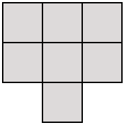
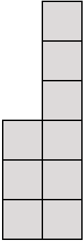
The shapes below are made up of identical squares.
Which shape covers the largest area?
 |
 |
 |
 |
|
|
|
|
|
`text{The first image has the highest number of squares (10)}`
`text{and therefore the largest area.}`
A road map shows some house numbers on Railway street.
Reg lives on Railway street in the house shown in the diagram.
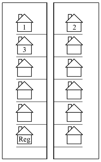
What is Reg's house number?
| `6` | `7` | `9` | `11` |
|
|
|
|
|
Chantelle showed this number on her calculator
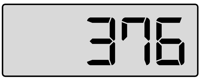
She changed it so that it became this number.
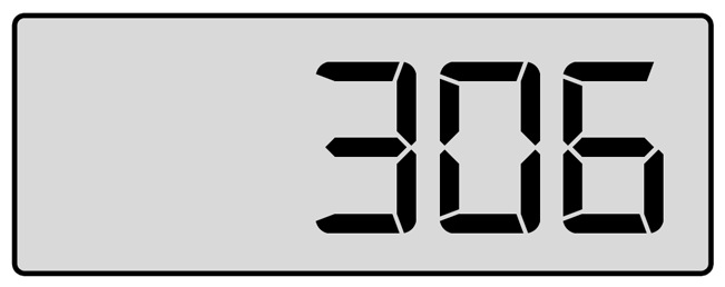
What did Chantelle do to change 376 to 306?
|
|
`text(added 7)` |
|
|
`text(subtracted 7)` |
|
|
`text(added 70)` |
|
|
`text(subtracted 70)` |
Rose called a restaurant on 3 November.
She booked dinner in exactly 3 weeks.
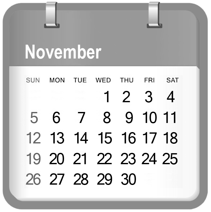
What date did Rose book the restaurant for?
|
|
`text(6 November)` |
|
|
`text(10 November)` |
|
|
`text(23 November)` |
|
|
`text(24 November)` |
Hasler spins the spinner below.
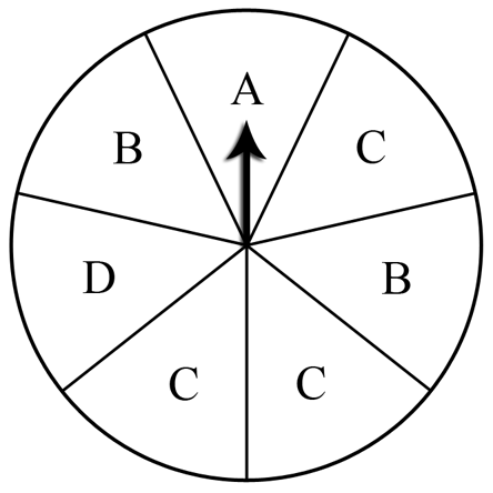
Which letter is the spinner most likely to land on?
| `text(A)` | `text(B)` | `text(C)` | `text(D)` |
|
|
|
|
|
This is a picture of a bunny using different shapes.
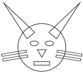
Which shape is not shown in the picture?
| `text(triangle)` | `text(circle)` | `text(rectangle)` | `text(square)` |
|
|
|
|
|
Miss Khan wrote this sentence on the board.
![]()
Which one of these matches Miss Khan's sentence?
|
|
`63 - 25 = 38` |
|
|
`63 + 25 = 38` |
|
|
`38 + 63 = 25` |
|
|
`38 - 25 = 63` |
| `37 + 18 =` |
|
| `43` | `54` | `55` | `515` |
|
|
|
|
|
How long is a quarter of an hour?
|
|
`text(15 seconds)` |
|
|
`text(25 seconds)` |
|
|
`text(30 seconds)` |
|
|
`text(25 minutes)` |
|
|
`text(15 minutes)` |
| `300 + 20 + 6 =` |
|
| `300\ 206` | `30\ 026` | `3206` | `326` |
|
|
|
|
|
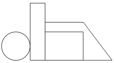
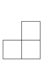
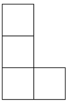
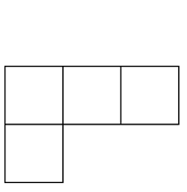
Six cubes are stacked together as shown.
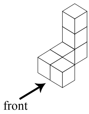
Which of these is the front view?
 |
 |
 |
 |
|
|
|
|
|
Which rectangle has three quarters shaded grey?
 |
 |
 |
 |
|
|
|
|
|
What time does the next ferry arrive?

|
|
four past six |
|
|
half past six |
|
|
four o'clock |
|
|
half past four |
|
|
half past five |
This repeating pattern is made by turning a square tile.

Which of these comes next in this pattern?
 |
 |
 |
 |
|
|
|
|
|
`text(The square is turned anti-clockwise each time.)`
`:.\ text(The next in the pattern is:)`
Six students line up side by side.
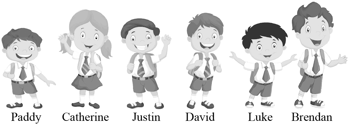
The teacher can make a line of shortest to tallest by swapping two students.
Which two students need to swap positions with each other?
|
|
`text(Catherine and Justin)` |
|
|
`text(Catherine and Luke)` |
|
|
`text(Justin and Luke)` |
|
|
`text(Paddy and Luke)` |
Pablo is part of the way through making a cube using plasticine balls and sticks, as shown below.
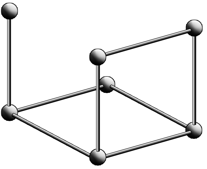
How many more sticks does Pablo need to finish the cube?
| `3` | `4` | `5` | `6` | `8` |
|
|
|
|
|
|
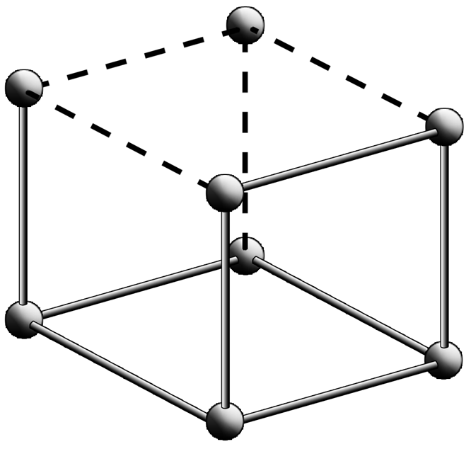
`text(The extra sticks needed = 4)`
Which clock shows a quarter past 6?
|
|
|
|
|
|
![]()
![]()
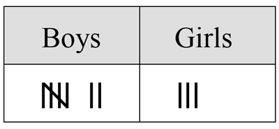
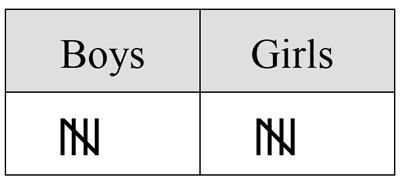
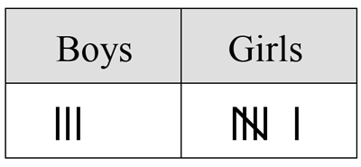
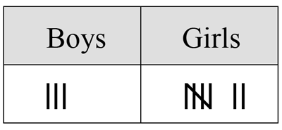
Kramer has 10 cousins, seven are girls and three are boys.
Which of these correctly shows Kramer's tally of his cousins?
 |
 |
 |
 |
|
|
|
|
|
A boat hire shop has 5 paddle boats.
Each paddle boat can fit 4 people in it.
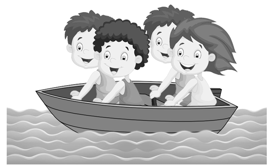
If all the paddle boats are hired out and have 4 people in them, how many people are in paddle boats altogether?
| `5` | `9` | `15` | `20` |
|
|
|
|
|
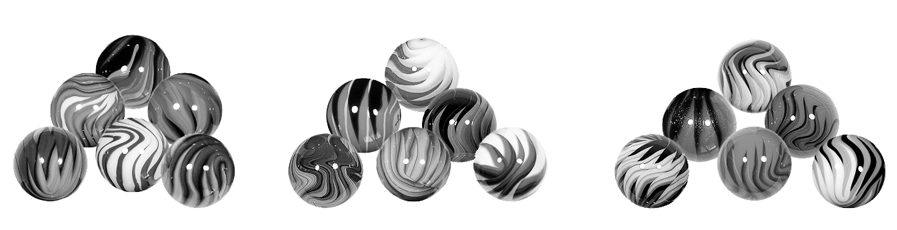
Carsten has 18 marbles in a bag.
To count the marbles, he puts them into groups of 3.
Which of the following shows the 18 marbles in groups of 3?
|
|
 |
|
|
 |
|
|
 |
|
|
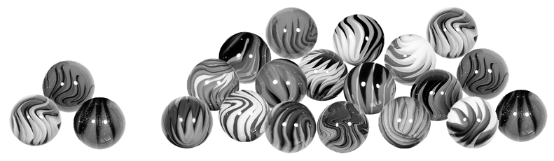 |
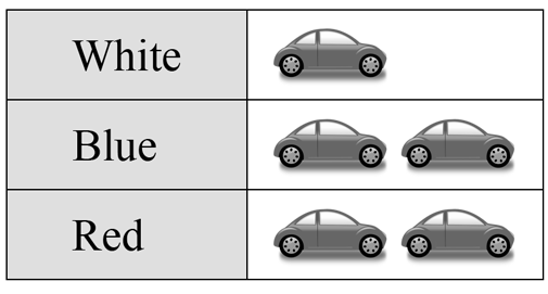
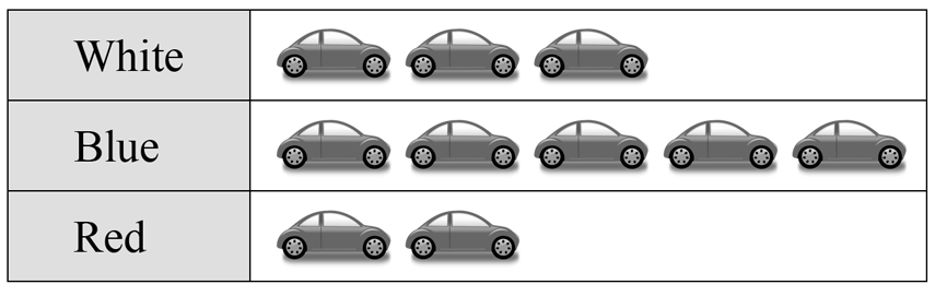
Cybil and Therese lived in different streets.
They were each counting different coloured cars that drove past their house one morning.
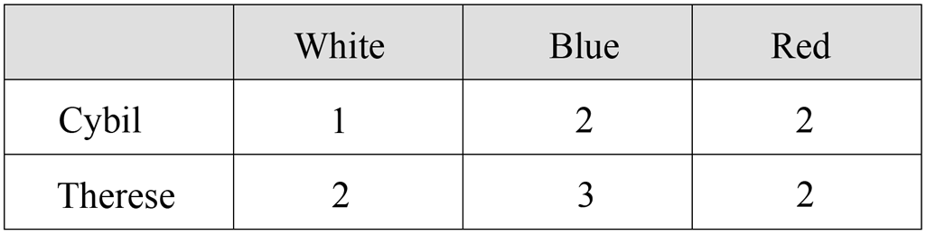
They drew a correct picture graph to show the number of coloured cars they saw altogether.
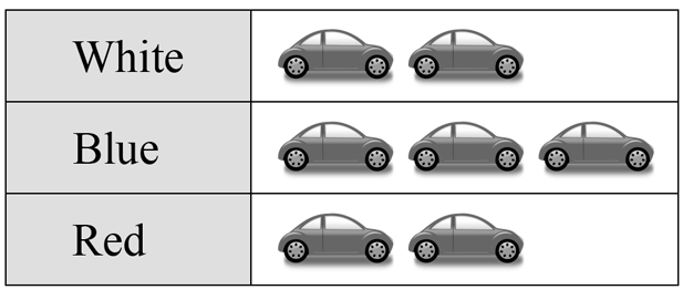
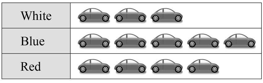
Which picture graph did they draw? ![]()
 |
 |
|
|
|
 |
 |
|
|
|
`text(Adding up the columns:)`
`text(White = 3, Blue = 5, Red = 4.)`
The world record for the most push-ups ever completed in one hour is three thousand and ninety-two.

The number of push-ups can be written as:
| `392` | `3092` | `3920` | `30\ 092` |
|
|
|
|
|
Rory played in a soccer team.
At training, 8 players were there but 4 could not make it.
How many players are in Rory's team?
| `4` | `8` | `11` | `12` |
|
|
|
|
|
This grid below shows a pattern.
Each row has a different shape.
Each column has different shading.
Some shapes are missing.

Which shape is missing from the bottom left corner of this grid?
 |
 |
 |
 |
|
|
|
|
|
Which of these gives the largest total?
| `40 + 500` | `6 + 600` | `30 + 600` | `7 + 500` |
|
|
|
|
|

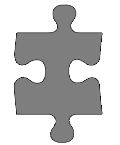
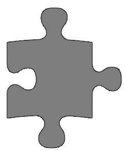
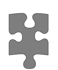
What shape is missing from this jigsaw?
 |
 |
 |
 |
|
|
|
|
|
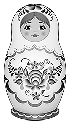
Cassandra has this doll
Sally has these dolls on a shelf.
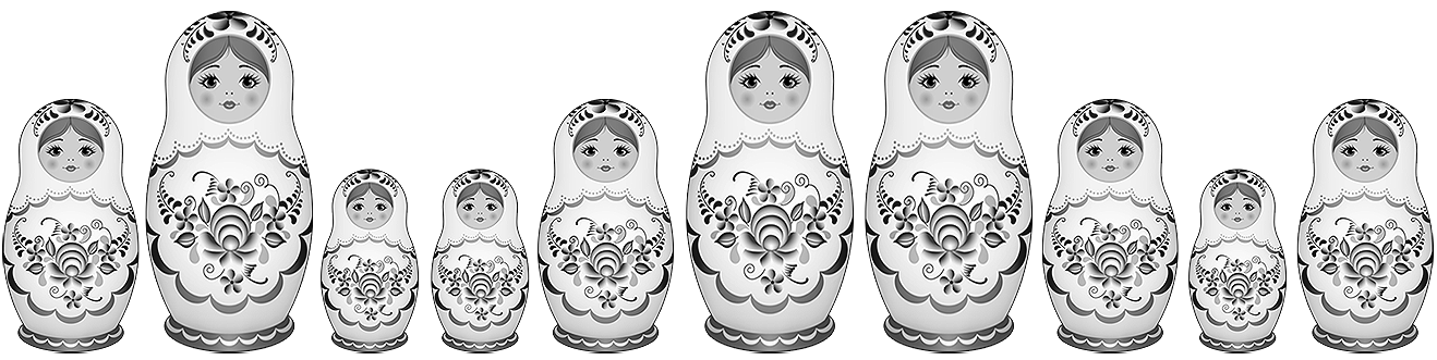
How many of Sally's dolls are the same height as Cassandra's doll?
| `6` | `5` | `4` | `3` |
|
|
|
|
|
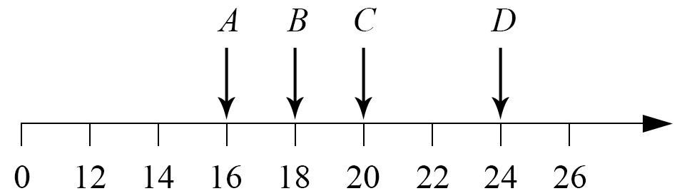
Which arrow points to the number that is halfway between 12 and 24?
| `A` | `B` | `C` | `D` |
|
|
|
|
|
Penny makes a pattern by turning a tile into different positions.

Which tile below belongs in position 4?
 |
 |
 |
 |
|
|
|
|
|
Cameron folded this piece of paper along the dotted lines to make a model.

Which of these models did Cameron make?
 |
 |
 |
 |
|
|
|
|
|
`text{The net folds into a triangular pyramid (which}`
`text{has a triangular base).}`
Andrew is travelling from Brisbane to Mackay.
He knows that it is more 968 kilometres but less than 986 kilometres.
Which of these could be the number of kilometres that Andrew has to travel?
| `946` | `964` | `984` | `988` |
|
|
|
|
|
Brianna recorded the colour of all cars that drove past her school during one hour for a class project.
The results were recorded in the table below.
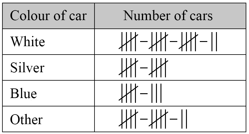
How many cars drove past Brianna's school in the hour?
Which clock shows half-past eight?
 |
 |
 |
 |
|
|
|
|
|
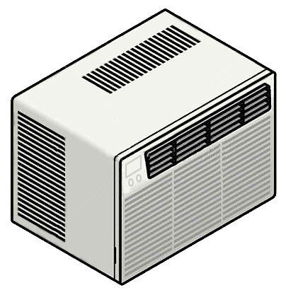
This 3D object pictured above is a
|
|
`text(cube)` |
|
|
`text(cylinder)` |
|
|
`text(rectangle)` |
|
|
`text(sphere)` |
Mary turns the arrow on her spinner.
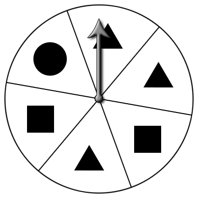
Which shape is the arrow least likely to stop on?
 |
||
|
|
|
|
![]()
![]()
| `44 + 28 =` |
The minute hand is not shown.
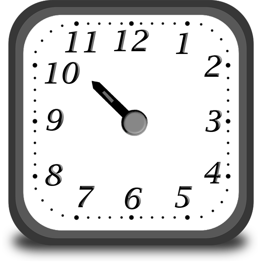
What time could this clock be displaying?
| `text(10 o'clock)` | `text(half past 10)` | `text(11 o'clock)` | `text(half past 11)` |
|
|
|
|
|
Which one of these equals 735?
 |
 |
 |
 |
|
|
|
|
|
Peter is packing soup cans into a box for charity.
The box is the same height as a soup can.
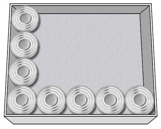
How many cans of soup will fit into the box?
| `8` | `9` | `15` | `20` |
|
|
|
|
|
This spreadsheet shows the names of athletes in three athletics clubs.

Which athlete's name is in cell B3?
Which of these nets will fold to make a triangular prism?
 |
 |
 |
 |
|
|
|
|
|
| `26 + 27 =` |
|
| `43` | `52` | `53` | `413` |
|
|
|
|
|
This table shows the three favourite subjects of four students.
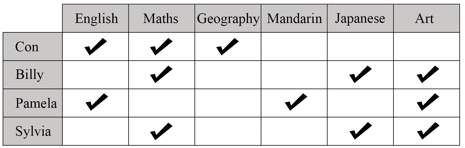
Which student chose Art but not Maths?
| `text(Con)` | `text(Billy)` | `text(Pamela)` | `text(Sylvia)` |
|
|
|
|
|