SmarterEd

Aussie Maths & Science Teachers: Save your time with SmarterEd

  • Login
  • Get Help
  • About

Statistics, 2ADV EQ-Bank 20

The weights of boxes of Brekky Bicks are normally distributed. The mean is 754 grams and the standard deviation is 2 grams.

  1. What is the `z`-score of a box of Brekky Bicks with a weight of 754 g?   (1 mark)

    --- 2 WORK AREA LINES (style=lined) ---

  2. What is the weight of a box that has a `z`-score of  –1?   (1 mark)

    --- 2 WORK AREA LINES (style=lined) ---

  3. Brekky Bicks boxes are labelled as having a weight of 750 g. What percentage of boxes will have a weight less than 750 g?   (2 marks)

    --- 4 WORK AREA LINES (style=lined) ---

Show Answers Only

a.    `0\ text{(mean)}`

b.    `752\ text(grams)`

c.    `text(2.5%)`

Show Worked Solution

a.    `text{z-score (754 g) = 0  (754 g is the mean)}`


b.    `ztext(-score)` `= (x-mu)/sigma`
`-1` `= (x-54)/2`
 `x-754` `= -2`
`x`  `= 752\ text(grams)`

 
c.
    `text{z-score (750)= (750-754)/2= -2`


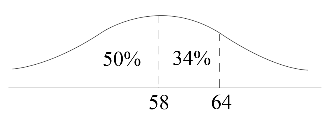
`:.\ text(Graph shows that 2.5% of boxes will weigh less than 750 g.)`
Filed Under: The Normal Distribution Tagged With: Band 3, Band 4, smc-7138-10-Single z-score

Statistics, 2ADV EQ-Bank 19

Two brands of light bulbs are being compared. For each brand, the life of the light bulbs, in hours, is normally distributed and described in the table below.

\begin{array} {|l|c|c|}
\hline
\rule{0pt}{2.5ex}  \rule[-1ex]{0pt}{0pt} & \quad \text{Mean} \quad & \text{Standard Deviation} \\
\hline
\rule{0pt}{2.5ex} \text{Brand A} \rule[-1ex]{0pt}{0pt} & 450 & 25 \\
\hline
\rule{0pt}{2.5ex} \text{Brand B} \rule[-1ex]{0pt}{0pt} & 500 & 50 \\
\hline
\end{array}

  1. One of the Brand B light bulbs has a life of 400 hours. 
  2. What is the `z`-score of the life of this light bulb?   (1 mark)

    --- 1 WORK AREA LINES (style=lined) ---

  3. A light bulb is considered defective if it lasts less than 400 hours. The following claim is made:
  4. ‘Brand A light bulbs are more likely to be defective than Brand B light bulbs.’
  5. Is this claim correct? Justify your answer, with reference to `z`-scores or standard deviations or the normal distribution.   (2 marks)

    --- 4 WORK AREA LINES (style=lined) ---

Show Answers Only

a.    `-2`

b.    `text(The claim is incorrect.)`

Show Worked Solution

a.    `z text{-score of Brand B bulb (400 hrs)}`

`= (x-mu)/sigma= (400-500)/50= -2`
 

b.   `z text{-score of Brand A bulb (400 hours)} =(400-450)/25=-2`

`text(S)text(ince the)\ z text(-score for both brands is –2, they are equally likely to be defective.)`

`:.\ text(The claim is incorrect.)`

Filed Under: The Normal Distribution Tagged With: Band 3, Band 4, smc-7138-10-Single z-score, smc-7138-30-Comparisons of Data Sets

Statistics, 2ADV EQ-Bank 16

The results of two class tests are normally distributed. The means and standard deviations of the tests are displayed in the table.

\begin{array} {|l|c|c|}
\hline
\rule{0pt}{2.5ex}  \rule[-1ex]{0pt}{0pt} & \quad \text{Test 1} \quad & \quad \text{Test 2} \quad \\
\hline
\rule{0pt}{2.5ex} \text{Mean} \rule[-1ex]{0pt}{0pt} & 60 & 58 \\
\hline
\rule{0pt}{2.5ex} \text{Standard Deviation} \rule[-1ex]{0pt}{0pt} & 6.2 & 6.0 \\
\hline
\end{array}

  1. Stuart scored 63 in Test 1 and 62 in Test 2. He thinks that he has performed better in Test 1. Do you agree? Justify your answer using appropriate calculations.   (2 marks)

    --- 5 WORK AREA LINES (style=lined) ---

  2. If 150 students sat for Test 2, how many students would you expect to have scored less than 64?   (2 marks)

    --- 4 WORK AREA LINES (style=lined) ---

Show Answers Only

a.    `text(Proof)\ \ text{(See Worked Solutions)}`

b.    `126`

Show Worked Solution

a.    `text(In Test 1:)\ \ mu = 60,\ sigma = 6.2`

`z text(-score)\ (63)= (x-mu)/sigma= (63-60)/6.2= 0.483…`

 
`text(In Test 2:)\ \ mu = 58,\ sigma = 6.0`

`z text(-score)\ (62)= (62-58)/6.0=0.666…`

`text(S) text(ince Stuart’s)\ z\ text(-score is higher in Test 2, his performance relative)`

`text(to the class is better despite his mark being slightly lower.)`
 

b.    `text(In Test 2:)`

`z text(-score)\ (64)= (64-58)/6= 1`

`text(84% have)\ z text(-score) < 1`

`:.\ text(# Students expected below 64) = text(84%) xx 150 = 126`

Filed Under: The Normal Distribution Tagged With: Band 3, Band 4, smc-7138-10-Single z-score, smc-7138-30-Comparisons of Data Sets

Statistics, 2ADV EQ-Bank 5 MC

A machine produces cylindrical pipes. The mean of the diameters of the pipes is 8 cm and the standard deviation is 0.04 cm.

Assuming a normal distribution, what percentage of cylindrical pipes produced will have a diameter less than 7.96 cm?

  1. `text(16%)`
  2. `text(32%)`
  3. `text(34%)`
  4. `text(68%)`
Show Answers Only

`A`

Show Worked Solution

`mu = 8\ text(cm)\ \ \ s = 0.04\ text(cm)`

`ztext{-score(7.96)}= (x-mu)/sigma= (7.96-8)/0.04=-1`
 

2UG 2015 20MC Answer

`:.\ text(% of pipes with a diameter less than 7.96 cm.)`

`=\ text(50%)-text(34%)`

`=\ text(16%)`

`=>A`

Filed Under: The Normal Distribution Tagged With: Band 4, smc-7138-10-Single z-score

Statistics, 2ADV S3 2025 HSC 23

  1. In a flock of 12 600 sheep, the ratio of males to females is \(1:20\).
  2. The weights of the male sheep are normally distributed with a mean of 76.2 kg and a standard deviation of 6.8 kg.
  3. In the flock, 15 of the male sheep each weigh more than \(x\) kg. 
  4. Find the value of \(x\).   (4 marks)

    --- 10 WORK AREA LINES (style=lined) ---

  5. The weights of the female sheep are also normally distributed but have a smaller mean and smaller standard deviation than the weights of male sheeр.
  6. Explain whether it could be expected that 300 of the females from the flock each weigh more than \(x\) kg, where \(x\) is the value found in part (a).   (1 mark)

    --- 5 WORK AREA LINES (style=lined) ---

Show Answers Only

a.   \(x=89.8 \ \text{kg}\)

b.    \(\text{Female sheep} \ \%=\dfrac{300}{12\,000}=0.025 \%\ (z \text{-score = 2)}\)

\(\text{Given} \ \ \bar{x}_f<\bar{x}_m \ \ \text{and} \ \ s_f<s_m\)

\(\text{Consider the value of}\ x_f\ \text{when \(z\)-score = 2}:\)

\(\Rightarrow x_f=\bar{x}_f+2 \times s_f \leq x_m\)

\(\therefore \ \text{It is not expected that  300 females weigh > 89.8 kg.}\)

Show Worked Solution

a.    \(12\,600 \ \text{sheep} \ \Rightarrow \ \text{male : female}=1:20\)

\(\text{Number of sheep in “1 part”} = \dfrac{12\,600}{21}=600\)

\(\Rightarrow \ \text{male : female}=600:12\,000\)

\(\text{male sheep} \ \%=\dfrac{15}{600}=0.025\%\)

\(z \text{-score }(0.025 \%)=2\)

\(\text{Using } \ z=\dfrac{x-\bar{x}}{s}, \ \text{find} \ \ x_m:\)

\(2\) \(=\dfrac{x_m-76.2}{6.8}\)  
\(x_m\) \(=76.2+2 \times 6.8=89.8 \ \text{kg}\)  

 
b. 
  \(\text{Female sheep} \ \%=\dfrac{300}{12\,000}=0.025 \%\ (z \text{-score = 2)}\)

\(\text{Given} \ \ \bar{x}_f<\bar{x}_m \ \ \text{and} \ \ s_f<s_m\)

\(\text{Consider the value of}\ x_f\ \text{when \(z\)-score = 2}:\)

\(\Rightarrow x_f=\bar{x}_f+2 \times s_f \leq x_m\)

\(\therefore \ \text{It is not expected that 300 females weigh > 89.8 kg.}\)

♦♦ Mean mark (b) 35%.

Filed Under: Normal Distribution, The Normal Distribution Tagged With: 2adv-std2-common, Band 4, Band 5, smc-7138-10-Single z-score, smc-995-10-Single z-score

Statistics, 2ADV S3 2025 HSC 8 MC

The minimum daily temperature, in degrees, of a town each year follows a normal distribution with its mean equal to its standard deviation. The minimum daily temperature was recorded over one year.

What percentage of the recorded minimum daily temperatures was above zero degrees?

  1. 16%
  2. 50%
  3. 68%
  4. 84%
Show Answers Only

\(D\)

Show Worked Solution

\(\text{Consider a possible example:}\)

\(\text{Let mean min daily temperature = 8°C}\)

\(\text{Std dev = 8°C}\)

\(z\text{-score (0°C)}\ =-1\)

\(\text{Percentage above 0°C} = 50+34=84\%\)

\(\Rightarrow D\)

♦ Mean mark 41%.

Filed Under: Normal Distribution, The Normal Distribution Tagged With: Band 4, smc-7138-10-Single z-score, smc-995-10-Single z-score

Statistics, 2ADV S3 2024 HSC 23

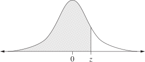
A random variable is normally distributed with mean 0 and standard deviation 1. The table gives the probability that this random variable is less than \(z\).

\begin{array} {|c|c|c|c|c|c|c|c|c|c|}
\hline
\rule{0pt}{2.5ex} z \rule[-1ex]{0pt}{0pt} & 0.6 & 0.7 & 0.8 & 0.9 & 1.0 & 1.1 & 1.2 & 1.3 & 1.4 \\
\hline
\rule{0pt}{2.5ex} \textit{Probability} \rule[-1ex]{0pt}{0pt} & 0.7257 & 0.7580 & 0.7881 & 0.8159 & 0.8413 & 0.8643 & 0.8849 & 0.9032 & 0.9192 \\
\hline
\end{array}

The probability values given in the table for different values of \(z\) are represented by the shaded area in the following diagram.
 

The scores in a university examination with a large number of candidates are normally distributed with mean 58 and standard deviation 15.

  1. By calculating a \(z\)-score, find the percentage of scores that are between 58 and 70.   (2 marks)

    --- 4 WORK AREA LINES (style=lined) ---

  2. Explain why the percentage of scores between 46 and 70 is twice your answer to part (a).   (1 mark)

    --- 2 WORK AREA LINES (style=lined) ---

  3. By using the values in the table above, find an approximate minimum score that a candidate would need to be placed in the top 10% of the candidates.   (2 marks)

    --- 4 WORK AREA LINES (style=lined) ---

Show Answers Only

a.   \(28.81%\)

b.   \(\text{Normal distribution is symmetrical about the mean (58).}\)

\(\text{Since 70 and 46 are both the same distance (12) from the mean, the percentage}\)

\(\text{of scores in this range will be twice the answer in part (a).}\)

c.   \(\text{Approx minimum score = 78%}\)

Show Worked Solution

a.   \(z\text{-score (58)}\ =\dfrac{x-\mu}{\sigma} = \dfrac{58-58}{15}=0\)

\(z\text{-score (70)}\ = \dfrac{70-58}{15}=0.8\)

\(\text{Using table:}\)

\(\text{% between 58–70}\ =0.7881-0.5=0.2881=28.81%\)
 

b.   \(\text{Normal distribution is symmetrical about the mean (58).}\)

\(\text{Since 70 and 46 are both the same distance (12) from the mean, the percentage}\)

\(\text{of scores in this range will be twice the answer in part (a).}\)
 

c.   \(z\text{-score 1.3 has a table value 0.9032}\)

\(1-0.9032=0.0968\ \Rightarrow\ \text{i.e. 9.68% of students score higher.}\)

\(\text{Find}\ x\ \text{for a}\ z\text{-score of 1.3:}\)

\(1.3\) \(=\dfrac{x-58}{15}\)  
\(x\) \(=1.3 \times 15 +58\)   
  \(=77.5\)  

 
\(\therefore\ \text{Approx minimum score = 78%}\)

Filed Under: Normal Distribution, The Normal Distribution Tagged With: 2adv-std2-common, Band 4, smc-7138-10-Single z-score, smc-7138-20-z-score Intervals, smc-7138-45-z-score tables, smc-995-10-Single z-score, smc-995-20-z-score Intervals, smc-995-45-z-score tables

Statistics, 2ADV S3 2023 HSC 23

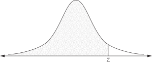
A random variable is normally distributed with a mean of 0 and a standard deviation of 1 . The table gives the probability that this random variable lies below `z` for some positive values of `z`.

The probability values given in the table are represented by the shaded area in the following diagram.
 

The weights of adult male koalas form a normal distribution with mean `mu` = 10.40 kg, and standard deviation `sigma` = 1.15 kg.

In a group of 400 adult male koalas, how many would be expected to weigh more than 11.93 kg?  (4 marks)

--- 8 WORK AREA LINES (style=lined) ---

Show Answers Only

`37\ text{koalas*}`

`text{*36 or 36.72 koalas would also receive full marks}`

Show Worked Solution
`ztext{-score (11.93)}` `=(x-mu)/sigma`  
  `=(11.93-10.4)/1.15`  
  `=1.330`  

 
`Ptext{(Koala weighs > 11.93 kg)}\ = P(z>1.330)`

`text{Using the table:}`

`P(z>1.33)` `=1-0.9082`  
  `=0.0918`  


`:.\ text{Expected koalas > 11.93 kg}` `=0.0918 xx 400`  
  `=36.72`  
  `=37\ text{koalas*}`  

 
`text{*36 or 36.72 koalas would also receive full marks}`

Filed Under: Normal Distribution, The Normal Distribution Tagged With: 2adv-std2-common, Band 4, smc-7138-10-Single z-score, smc-7138-45-z-score tables, smc-995-10-Single z-score, smc-995-45-z-score tables

Statistics, 2ADV S3 2021 HSC 32

In a particular city, the heights of adult females and the heights of adult males are each normally distributed.

Information relating to two females from that city is given in Table 1.
 

The means and standard deviations of adult females and males, in centimetres, are given in Table 2.


A selected male is taller than 84% of the population of adult males in this city.

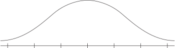
By first labelling the normal distribution curve below with the heights of the two females given in Table 1, calculate the height of the selected male, in centimetres, correct to two decimal places.  (4 marks)


--- 6 WORK AREA LINES (style=lined) ---

Show Answers Only

`178.95 \ text{cm}`

Show Worked Solution


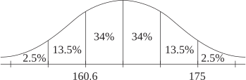
`z text{-score (175 cm, female)} = 2`

♦ Mean mark 41%.

`z text{-score (160.6 cm, female)} = -1`
 

`text{Find} \ mu \ text{of female heights:}`

`mu – sigma` `= 160.6`  
`mu + 2sigma` `= 175`  
`3 sigma` `= 175 – 160.6`  
`sigma` `= 14.4/3`  
  `= 4.8 \ text{cm}`  
`:. \ mu` `= 165.4 \ text{cm}`  


`text{Selected male’s height has} \ z text{-score} = 1`

`mu text{(male)} = 1.05 times 165.4 = 173.67`

`sigma \ text{(male)} = 1.1 times 4.8 = 5.28`


`:. \ text{Actual male height}` `= 173.67 + 5.28`  
  `= 178.95 \ text{cm}`  

Filed Under: Normal Distribution, The Normal Distribution Tagged With: Band 5, smc-7138-10-Single z-score, smc-7138-30-Comparisons of Data Sets, smc-995-10-Single z-score, smc-995-30-Comparisons of Data Sets

Copyright © 2014–2026 SmarterEd.com.au · Log in