SmarterEd

Aussie Maths & Science Teachers: Save your time with SmarterEd

  • Login
  • Get Help
  • About

Statistics, 2ADV EQ-Bank 34

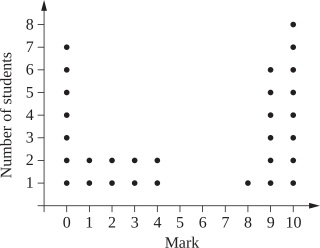
All the students in a class of 30 did a test.

The marks, out of 10, are shown in the dot plot.
 

  1. Find the median test mark.   (1 mark)

    --- 1 WORK AREA LINES (style=lined) ---

  2. The mean test mark is 5.4. The standard deviation of the test marks is 4.22.
  3. Using the dot plot, calculate the percentage of the marks which lie within one standard deviation of the mean.   (2 marks)

    --- 4 WORK AREA LINES (style=lined) ---

  4. A student states that for any data set, 68% of the scores should lie within one standard deviation of the mean. With reference to the dot plot, explain why the student’s statement is NOT relevant in this context.   (1 mark)

    --- 2 WORK AREA LINES (style=lined) ---
Show Answers Only

i.    `6`

ii.   `text(43%)`

iii.  `text(The statement assumes the data is normally distributed which is incorrect.)`

Show Worked Solution
♦ Mean mark (i) 50%.
♦♦Mean mark (ii) 34%.

i.    `text(Median)= text(15th + 16th score)/2= (4 + 8)/2= 6`
 

ii.   `text(Lower limit) = 5.4-4.22 = 1.18`

`text(Upper limit) = 5.4 + 4.22 = 9.62`

`:.\ text(Percentage in between)`

`= 13/30 xx 100`

`= 43.33…`

`= 43text{%  (nearest %)}`
 

iii.   `text(The statement assumes the data is normally distributed.)`

♦♦♦ Mean mark (iii) 13%.

`text(This is incorrect in this case.)`

Filed Under: The Normal Distribution Tagged With: Band 3, Band 4, Band 5, smc-7138-20-z-score Intervals, smc-7138-30-Comparisons of Data Sets

Statistics, 2ADV EQ-Bank 29

The results of two tests are normally distributed. The mean and standard deviation for each test are displayed in the table.

\begin{array} {|l|c|c|}
\hline
\rule{0pt}{2.5ex}  \rule[-1ex]{0pt}{0pt} & \text{Mathematics} & \quad \text{English} \quad \\
\hline
\rule{0pt}{2.5ex} \quad \mu \quad \rule[-1ex]{0pt}{0pt} & 70 & 75 \\
\hline
\rule{0pt}{2.5ex} \quad \sigma \rule[-1ex]{0pt}{0pt} & 6.5 & 8 \\
\hline
\end{array}

Kristoff scored 74 in Mathematics and 80 in English. He claims that he has performed better in English.

Is Kristoff correct? Justify your answer using appropriate calculations.   (2 marks)

--- 6 WORK AREA LINES (style=lined) ---
Show Answers Only

`text(He is correct.)`

Show Worked Solution

`text(In Maths:)`

♦ Mean mark 44%.

`ztext{-score (74)}= (x-mu)/sigma= (74-70)/6.5= 0.6153…`

`text(In English:)`

`ztext{-score (80)}=(80-75)/8= 0.625`
 

`text(Kristoff’s)\ ztext(-score in English is higher than his)\ z text(-score in Maths.)`

`:.\ text(He is correct. He performed better in English.)`

Filed Under: The Normal Distribution Tagged With: Band 4, smc-7138-30-Comparisons of Data Sets

Statistics, 2ADV EQ-Bank 19

Two brands of light bulbs are being compared. For each brand, the life of the light bulbs, in hours, is normally distributed and described in the table below.

\begin{array} {|l|c|c|}
\hline
\rule{0pt}{2.5ex}  \rule[-1ex]{0pt}{0pt} & \quad \text{Mean} \quad & \text{Standard Deviation} \\
\hline
\rule{0pt}{2.5ex} \text{Brand A} \rule[-1ex]{0pt}{0pt} & 450 & 25 \\
\hline
\rule{0pt}{2.5ex} \text{Brand B} \rule[-1ex]{0pt}{0pt} & 500 & 50 \\
\hline
\end{array}

  1. One of the Brand B light bulbs has a life of 400 hours. 
  2. What is the `z`-score of the life of this light bulb?   (1 mark)

    --- 1 WORK AREA LINES (style=lined) ---
  3. A light bulb is considered defective if it lasts less than 400 hours. The following claim is made:
  4. ‘Brand A light bulbs are more likely to be defective than Brand B light bulbs.’
  5. Is this claim correct? Justify your answer, with reference to `z`-scores or standard deviations or the normal distribution.   (2 marks)

    --- 4 WORK AREA LINES (style=lined) ---
Show Answers Only

a.    `-2`

b.    `text(The claim is incorrect.)`

Show Worked Solution

a.    `z text{-score of Brand B bulb (400 hrs)}`

`= (x-mu)/sigma= (400-500)/50= -2`
 

b.   `z text{-score of Brand A bulb (400 hours)} =(400-450)/25=-2`

`text(S)text(ince the)\ z text(-score for both brands is –2, they are equally likely to be defective.)`

`:.\ text(The claim is incorrect.)`

Filed Under: The Normal Distribution Tagged With: Band 3, Band 4, smc-7138-10-Single z-score, smc-7138-30-Comparisons of Data Sets

Statistics, 2ADV EQ-Bank 16

The results of two class tests are normally distributed. The means and standard deviations of the tests are displayed in the table.

\begin{array} {|l|c|c|}
\hline
\rule{0pt}{2.5ex}  \rule[-1ex]{0pt}{0pt} & \quad \text{Test 1} \quad & \quad \text{Test 2} \quad \\
\hline
\rule{0pt}{2.5ex} \text{Mean} \rule[-1ex]{0pt}{0pt} & 60 & 58 \\
\hline
\rule{0pt}{2.5ex} \text{Standard Deviation} \rule[-1ex]{0pt}{0pt} & 6.2 & 6.0 \\
\hline
\end{array}

  1. Stuart scored 63 in Test 1 and 62 in Test 2. He thinks that he has performed better in Test 1. Do you agree? Justify your answer using appropriate calculations.   (2 marks)

    --- 5 WORK AREA LINES (style=lined) ---

  2. If 150 students sat for Test 2, how many students would you expect to have scored less than 64?   (2 marks)

    --- 4 WORK AREA LINES (style=lined) ---

Show Answers Only

a.    `text(Proof)\ \ text{(See Worked Solutions)}`

b.    `126`

Show Worked Solution

a.    `text(In Test 1:)\ \ mu = 60,\ sigma = 6.2`

`z text(-score)\ (63)= (x-mu)/sigma= (63-60)/6.2= 0.483…`

 
`text(In Test 2:)\ \ mu = 58,\ sigma = 6.0`

`z text(-score)\ (62)= (62-58)/6.0=0.666…`

`text(S) text(ince Stuart’s)\ z\ text(-score is higher in Test 2, his performance relative)`

`text(to the class is better despite his mark being slightly lower.)`
 

b.    `text(In Test 2:)`

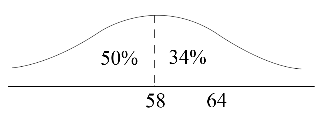
`z text(-score)\ (64)= (64-58)/6= 1`

`text(84% have)\ z text(-score) < 1`

`:.\ text(# Students expected below 64) = text(84%) xx 150 = 126`

Filed Under: The Normal Distribution Tagged With: Band 3, Band 4, smc-7138-10-Single z-score, smc-7138-30-Comparisons of Data Sets

Statistics, 2ADV S3 2024 HSC 3 MC

Pia's marks in Year 10 assessments are shown. The scores for each subject were normally distributed.

\begin{array}{|l|c|c|c|}
\hline & \textit {Pia's mark} & \textit {Year 10 mean} & \textit {Year 10 standard} \\
&&&\textit {deviation}\\
\hline \text {English} & 78 & 66 & 6 \\
\hline \text {Mathematics} & 80 & 71 & 10 \\
\hline \text {Science} & 77 & 70 & 15 \\
\hline \text {History} & 85 & 72 & 9 \\
\hline
\end{array}

In which subject did Pia perform best in comparison with the rest of Year 10?

  1. English
  2. Mathematics
  3. Science
  4. History
Show Answers Only

\(A\)

Show Worked Solution

\(\text {Consider the z-score of each option:}\)

\(z \text {-score (English)}=\dfrac{78-66}{6}=2\)

\(z \text {-score (Maths)}=\dfrac{80-71}{10}=0.9\)

\(z \text {-score (Science) }=\dfrac{77-70}{15}=0.46 \ldots\)

\(z \text {-score (History})=\dfrac{85-72}{9}=1.4 \ldots\)

\(\Rightarrow A\)

Filed Under: Normal Distribution, The Normal Distribution Tagged With: 2adv-std2-common, Band 3, smc-7138-30-Comparisons of Data Sets, smc-995-30-Comparisons of Data Sets

Statistics, 2ADV S3 2021 HSC 32

In a particular city, the heights of adult females and the heights of adult males are each normally distributed.

Information relating to two females from that city is given in Table 1.
 

The means and standard deviations of adult females and males, in centimetres, are given in Table 2.


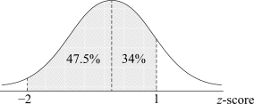
A selected male is taller than 84% of the population of adult males in this city.

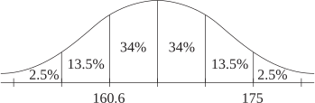
By first labelling the normal distribution curve below with the heights of the two females given in Table 1, calculate the height of the selected male, in centimetres, correct to two decimal places.  (4 marks)


--- 6 WORK AREA LINES (style=lined) ---

Show Answers Only

`178.95 \ text{cm}`

Show Worked Solution


`z text{-score (175 cm, female)} = 2`

♦ Mean mark 41%.

`z text{-score (160.6 cm, female)} = -1`
 

`text{Find} \ mu \ text{of female heights:}`

`mu – sigma` `= 160.6`  
`mu + 2sigma` `= 175`  
`3 sigma` `= 175 – 160.6`  
`sigma` `= 14.4/3`  
  `= 4.8 \ text{cm}`  
`:. \ mu` `= 165.4 \ text{cm}`  


`text{Selected male’s height has} \ z text{-score} = 1`

`mu text{(male)} = 1.05 times 165.4 = 173.67`

`sigma \ text{(male)} = 1.1 times 4.8 = 5.28`


`:. \ text{Actual male height}` `= 173.67 + 5.28`  
  `= 178.95 \ text{cm}`  

Filed Under: Normal Distribution, The Normal Distribution Tagged With: Band 5, smc-7138-10-Single z-score, smc-7138-30-Comparisons of Data Sets, smc-995-10-Single z-score, smc-995-30-Comparisons of Data Sets

Statistics, 2ADV S3 2020 HSC 28

In a particular country, the hourly rate of pay for adults who work is normally distributed with a mean of $25 and a standard deviation of $5.

  1. Two adults who both work are chosen at random.


    Find the probability that at least one of them earns between $15 and $30 per hour.  (3 marks)

    --- 6 WORK AREA LINES (style=lined) ---

  2. The number of adults who work is equal to three times the number of adults who do not work.


    One adult is chosen at random.


    Find the probability that the chosen adult works and earn more than $25 per hour.  (2 marks)

    --- 4 WORK AREA LINES (style=lined) ---

Show Answers Only
  1. `0.965775`
  2. `3/8`
Show Worked Solution

`ztext(-score)\ ($15) = (x – mu)/sigma = (15 – 25)/5 = −2`

♦ Mean mark part (a) 40%.

`ztext(-score)\ ($30) = (30 -25)/5 = 1`
 

`text(Percentage of scores where)\  −2 <= z <= 1`

`= 81.5text(%)`
 

`P(text(at least one earns between $15 – $30))`

`= 1 – P(text(neither))`

`= 1 – (1-0.815)^2`

`=1-0.185^2`

`= 0.965775`


b.
   `P(text(works)) = 3/4, \ P(text(earns) > $25) = 1/2`

`:. P(text(works and earns) > $25)`

`= 3/4 xx 1/2`

`= 3/8`

Filed Under: Normal Distribution, The Normal Distribution Tagged With: Band 4, Band 5, smc-7138-20-z-score Intervals, smc-7138-30-Comparisons of Data Sets, smc-995-20-z-score Intervals, smc-995-30-Comparisons of Data Sets

Statistics, 2ADV S3 2020 HSC 3 MC

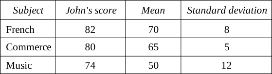
John recently did a class test in each of three subjects. The class scores on each test were normally distributed.

The table shows the subjects and John's scores as well as the mean and standard deviation of the class scores on each test.


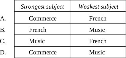
Relative to the rest of class, which row of the table below shows John's strongest subject and his weakest subject?
 

Show Answers Only

`A`

Show Worked Solution

`text(Calculate the)\ ztext(-score of each subject:)`

`ztext{-score (French)} = frac(82 – 70)(8) = 1.5`

`ztext{-score (Commerce)} = frac(80 – 65)(5) = 3.0`

`ztext{-score (Music)} = frac(74 – 50)(12) = 2.0`

 
`therefore \ text{Commerce is strongest, French is weakest}`

`=> \ A`

Filed Under: Normal Distribution, The Normal Distribution Tagged With: 2adv-std2-common, Band 4, common-content, smc-7138-30-Comparisons of Data Sets, smc-995-30-Comparisons of Data Sets

Copyright © 2014–2026 SmarterEd.com.au · Log in