Data was collected to investigate the behaviour of tides in Sydney Harbour. There are usually two high tides and two low tides each day. The variables in this study were: Table 1 displays the data collected for a sample of 14 consecutive days in February 2021. Table 1 \begin{array}{|c|c|c|} --- 2 WORK AREA LINES (style=lined) --- --- 2 WORK AREA LINES (style=lined) --- --- 0 WORK AREA LINES (style=lined) --- \begin{array}{|c|c|c|c|c|} --- 4 WORK AREA LINES (style=lined) --- --- 0 WORK AREA LINES (style=lined) --- a.i. \(\text{Mean = 1.6}\) a.ii. \(\text{Std dev = 0.185}\) b. c. \(IQR (LLT) = 0.65-0.39=0.26\) \(\text{Lower fence}\ =Q_1-1.5 \times IQR = 0.39-1.5 \times o.26=0\) \(\text{Since 0.22 > 0, 0.22 is not an outlier.}\) d. \(HHT = 2.130 + (-1.054) \times LLT\) a.i. \(\text{Mean = 1.6}\) a.ii. \(\text{Std dev = 0.185}\) b. \(\text{Order \(HHT\) data:}\) \(1.42, 1.42, 1.42, [1.42], 1,44, 1.47, 1.55 | 1.55, 1.64, 1.65, [1.74],\) \(1.83, 1.90, 1.92\) \(\text{High = 1.92, Low = 1.42, \(Q_1=1.42, Q_3=1.74\), Median = 1.55}\) \(\text{Lower fence}\ =Q_1-1.5 \times IQR = 0.39-1.5 \times 0.26=0\) \(\text{Since 0.22 > 0, 0.22 is not an outlier.}\) d. \(HHT\ \text{is the response \((y)\) variable.}\) \(\text{By CAS:}\) \(HHT = 2.130 + (-1.054) \times LLT\)
\hline
\rule{0pt}{2.5ex}\ \ \ \textit{Day}\ \ \ \rule[-1ex]{0pt}{0pt}& \textit{LLT (m)} & \textit{HHT (m)}\\
\hline \rule{0pt}{2.5ex}1 \rule[-1ex]{0pt}{0pt}& 0.43 & 1.65 \\
\hline \rule{0pt}{2.5ex}2 \rule[-1ex]{0pt}{0pt}& 0.49 & 1.55 \\
\hline \rule{0pt}{2.5ex}3 \rule[-1ex]{0pt}{0pt}& 0.55 & 1.44 \\
\hline \rule{0pt}{2.5ex}4 \rule[-1ex]{0pt}{0pt}& 0.61 & 1.42 \\
\hline \rule{0pt}{2.5ex}5 \rule[-1ex]{0pt}{0pt}& 0.68 & 1.42 \\
\hline \rule{0pt}{2.5ex}6 \rule[-1ex]{0pt}{0pt}& 0.73 & 1.42 \\
\hline \rule{0pt}{2.5ex}7 \rule[-1ex]{0pt}{0pt}& 0.72 & 1.42 \\
\hline \rule{0pt}{2.5ex}8 \rule[-1ex]{0pt}{0pt}& 0.65 & 1.47 \\
\hline \rule{0pt}{2.5ex}9 \rule[-1ex]{0pt}{0pt}& 0.57 & 1.55 \\
\hline \rule{0pt}{2.5ex}10 \rule[-1ex]{0pt}{0pt}& 0.48 & 1.64 \\
\hline \rule{0pt}{2.5ex}11 \rule[-1ex]{0pt}{0pt}& 0.39 & 1.74 \\
\hline \rule{0pt}{2.5ex}12 \rule[-1ex]{0pt}{0pt}& 0.30 & 1.83 \\
\hline \rule{0pt}{2.5ex}13 \rule[-1ex]{0pt}{0pt}& 0.25 & 1.90 \\
\hline \rule{0pt}{2.5ex}14 \rule[-1ex]{0pt}{0pt}& 0.22 & 1.92 \\
\hline
\end{array}

\hline \rule{0pt}{2.5ex}\textbf{Minimum} \rule[-1ex]{0pt}{0pt}& \ \ \textbf{Q1} \ \ & \textbf{Median} & \ \ \textbf{Q3} \ \ & \textbf{Maximum} \\
\hline \rule{0pt}{2.5ex}0.22 \rule[-1ex]{0pt}{0pt}& 0.39 & 0.52 & 0.65 & 0.73 \\
\hline
\end{array}
![]()

c. \(IQR (LLT) = 0.65-0.39=0.26\)
Data Analysis, GEN1 2024 NHT 9-10 MC
The scatterplot below shows the average annual income, in dollars, plotted against life expectancy, in years, for 42 countries in 2020.
A least squares line has been fitted to the scatterplot.
The coefficient of determination is 0.306.

Question 9
The equation of the least squares line is closest to
- income \(=-19\,000+345 \times\) life expectancy
- income \(=-19\,250+355 \times\) life expectancy
- income \(=-19\,500+365 \times\) life expectancy
- income \(=-19\,750+375 \times\) life expectancy
- income \(=-20\,000+385 \times\) life expectancy
Question 10
Which one of the following statements is true?
- The value of the correlation coefficient is 0.306
- There are more data points above the least squares line than below.
- 30.6% of the variation in annual income is not explained by the variation in life expectancy.
- The country with the longest life expectancy has a positive residual associated with it.
- Using the least squares line to predict the annual income of a country whose citizens have a life expectancy of 54 years is an example of extrapolation.
Data Analysis, GEN1 2024 NHT 8 MC
A class investigation considered 20 countries and any association between the birth rate, per 1000 people, and the life expectancy, in years.
Students were given the following table of summary statistics.

Scatterplots A, B, C, D and E show attempts by five students to fit the calculated least squares line to a scatterplot of the original data.
Which one of these attempts has been completed correctly?


Data Analysis, GEN2 2024 VCAA 1
Table 1 lists the Olympic year, \(\textit{year}\), and the gold medal-winning height for the men's high jump, \(\textit{Mgold}\), in metres, for each Olympic Games held from 1928 to 2020. No Olympic Games were held in 1940 or 1944, and the 2020 Olympic Games were held in 2021. Table 1 \begin{array}{|c|c|} --- 1 WORK AREA LINES (style=lined) --- --- 2 WORK AREA LINES (style=lined) --- --- 3 WORK AREA LINES (style=lined) --- --- 0 WORK AREA LINES (style=lined) --- --- 0 WORK AREA LINES (style=lined) --- --- 4 WORK AREA LINES (style=lined) --- a.i. \(2.39\) a.ii. \(50\%\) b. \(0.8\) c. d. e. \(\text{A coefficient of determination of 85.7% shows the variation in}\) \(\text{the}\ Mgold\ \text{that is explained by the variation in the }year.\) a.i. \(2.39\) a.ii. \(\dfrac{11}{22}=50\%\) \(Q_1=2.12, \ Q_3=2.36\) \(\text{Min}\ =1.94, \ \text{Max}\ =2.39\) e. \(\text{A coefficient of determination of 85.7% shows the variation in}\) \(\text{the}\ Mgold\ \text{that is explained by the variation in the }year.\)
\hline \quad \textit{year} \quad & \textit{Mgold}\,\text{(m)} \\
\hline 1928 & 1.94 \\
\hline 1932 & 1.97 \\
\hline 1936 & 2.03 \\
\hline 1948 & 1.98 \\
\hline 1952 & 2.04 \\
\hline 1956 & 2.12 \\
\hline 1960 & 2.16 \\
\hline 1964 & 2.18 \\
\hline 1968 & 2.24 \\
\hline 1972 & 2.23 \\
\hline 1976 & 2.25 \\
\hline 1980 & 2.36 \\
\hline 1984 & 2.35 \\
\hline 1988 & 2.38 \\
\hline 1992 & 2.34 \\
\hline 1996 & 2.39 \\
\hline 2000 & 2.35 \\
\hline 2004 & 2.36 \\
\hline 2008 & 2.36 \\
\hline 2012 & 2.33 \\
\hline 2016 & 2.38 \\
\hline 2020 & 2.37 \\
\hline
\end{array}

![]()
Show Answers Only

![]() Show Worked Solution
Show Worked Solution
b.
\(z\)
\(=\dfrac{x-\overline x}{s_x}\)
\(=\dfrac{2.35-2.23}{0.15}\)
\(=0.8\)
c. \(Q_2=\dfrac{2.33+2.25}{2}=2.29\)

Data Analysis, GEN1 2024 VCAA 8 MC
The scatterplot below displays the average number of female athletes per competing nation, females, against the number of the Summer Olympic Games, number, from the first Olympic Games, in 1896, to the 29th Olympic Games, held in 2021.
A least squares line has been fitted to the scatterplot.

The equation of the least squares line is closest to
- \(females =-4.87+1.02 \times number\)
- \( females =-3.39+0.91 \times number\)
- \(number =-3.39+0.91 \times females\)
- \(number =-0.91+3.39 \times females\)
Data Analysis, GEN1 2022 VCAA 12-14 MC
The scatterplot below displays the body length, in centimetres, of 17 crocodiles, plotted against their head length, in centimetres. A least squares line has been fitted to the scatterplot. The explanatory variable is head length.

Question 12
The equation of the least squares line is closest to
- head length = –40 + 7 × body length
- body length = –40 + 7 × head length
- head length = 168 + 7 × body length
- body length = 168 – 40 × head length
- body length = 7 + 168 × head length
Question 13
The median head length of the 17 crocodiles, in centimetres, is closest to
- 49
- 51
- 54
- 300
- 345
Question 14
The correlation coefficient \(r\) is equal to 0.963
The percentage of variation in body length that is not explained by the variation in head length is closest to
- 0.9%
- 3.7%
- 7.3%
- 92.7%
- 96.3%
Data Analysis, GEN2 2023 VCAA 1
Data was collected to investigate the use of electronic images to automate the sizing of oysters for sale. The variables in this study were: The data collected for a sample of 15 oysters is displayed in the table. --- 1 WORK AREA LINES (style=lined) --- --- 1 WORK AREA LINES (style=lined) --- --- 1 WORK AREA LINES (style=lined) --- --- 1 WORK AREA LINES (style=lined) --- --- 0 WORK AREA LINES (style=lined) --- --- 4 WORK AREA LINES (style=lined) --- --- 4 WORK AREA LINES (style=lined) ---

the median weight of the large oysters in this sample. (1 mark)
Complete the following sentence by filling in the blank space provided. (1 mark)
This equation predicts that, on average, each 10 g increase in the weight of an oyster is associated with a ________________ cm³ increase in its volume.
Data Analysis, GEN1 2023 VCAA 9 MC
A least squares line can be used to model the birth rate (children per 1000 population) in a country from the average daily food energy intake (megajoules) in that country.
When a least squares line is fitted to data from a selection of countries it is found that:
-
- for a country with an average daily food energy intake of 8.53 megajoules, the birth rate will be 32.2 children per 1000 population
- for a country with an average daily food energy intake of 14.9 megajoules, the birth rate will be 9.9 children per 1000 population.
The slope of this least squares line is closest to
- \(-4.7\)
- \(-3.5\)
- \(-0.29\)
- \(2.7\)
- \(25\)
CORE, FUR1 2021 VCAA 10 MC
Oscar walked for nine consecutive days. The time, in minutes, that Oscar spent walking on each day is shown in the table below.

At least squares line is fitted to the data.
The equation of this line predicts that on day 10 the time Oscar spends walking will be the same as the time he spent walking on
- day 3
- day 4
- day 6
- day 8
- day 9
CORE, FUR2 2020 VCAA 6
The table below shows the mean age, in years, and the mean height, in centimetres, of 648 women from seven different age groups.

- What was the difference, in centimetres, between the mean height of the women in their twenties and the mean height of the women in their eighties? (1 mark)
--- 1 WORK AREA LINES (style=lined) ---
A scatterplot displaying this data shows an association between the mean height and the mean age of these women. In an initial analysis of the data, a line is fitted to the data by eye, as shown.

- Describe this association in terms of strength and direction. (1 mark)
--- 1 WORK AREA LINES (style=lined) ---
- The line on the scatterplot passes through the points (20,168) and (85,157).
Using these two points, determine the equation of this line. Write the values of the intercept and the slope in the appropriate boxes below.
Round your answers to three significant figures. (1 mark)
--- 0 WORK AREA LINES (style=lined) ---
| mean height = |
|
+ |
|
× mean age |
- In a further analysis of the data, a least squares line was fitted.
The associated residual plot that was generated is shown below.

The residual plot indicates that the association between the mean height and the mean age of women is non-linear.
The data presented in the table in part a is repeated below. It can be linearised by applying an appropriate transformation to the variable mean age.

Apply an appropriate transformation to the variable mean age to linearise the data. Fit a least squares line to the transformed data and write its equation below.
Round the values of the intercept and the slope to four significant figures. (2 marks)
--- 5 WORK AREA LINES (style=lined) ---

CORE, FUR2 2020 VCAA 4
The age, in years, body density, in kilograms per litre, and weight, in kilograms, of a sample of 12 men aged 23 to 25 years are shown in the table below.
| Age (years) |
Body density |
Weight |
|
| 23 | 1.07 | 70.1 | |
| 23 | 1.07 | 90.4 | |
| 23 | 1.08 | 73.2 | |
| 23 | 1.08 | 85.0 | |
| 24 | 1.03 | 84.3 | |
| 24 | 1.05 | 95.6 | |
| 24 | 1.07 | 71.7 | |
| 24 | 1.06 | 95.0 | |
| 25 | 1.07 | 80.2 | |
| 25 | 1.09 | 87.4 | |
| 25 | 1.02 | 94.9 | |
| 25 | 1.09 | 65.3 |
- For these 12 men, determine
- i. their median age, in years. (1 mark)
--- 2 WORK AREA LINES (style=lined) ---
- ii. the mean of their body density, in kilograms per litre. (1 mark)
--- 2 WORK AREA LINES (style=lined) ---
- A least squares line is to be fitted to the data with the aim of predicting body density from weight.
- i. Name the explanatory variable for this least squares line. (1 mark)
--- 1 WORK AREA LINES (style=lined) ---
- ii. Determine the slope of this least squares line.
- Round your answer to three significant figures. (1 mark)
--- 1 WORK AREA LINES (style=lined) ---
- What percentage of the variation in body density can be explained by the variation in weight?
- Round your answer to the nearest percentage. (1 mark)
--- 2 WORK AREA LINES (style=lined) ---
Data Analysis, GEN2 2019 NHT 3
The life span, in years, and gestation period, in days, for 19 types of mammals are displayed in the table below.

- A least squares line that enables life span to be predicted from gestation period is fitted to this data.
- Name the explanatory variable in the equation of this least squares line. (1 mark)
--- 1 WORK AREA LINES (style=lined) ---
- Determine the equation of the least squares line in terms of the variables life span and gestation period.
- Round the numbers representing the intercept and slope to three significant figures. (2 marks)
--- 2 WORK AREA LINES (style=lined) ---
- Write the value of the correlation rounded to three decimal places. (1 mark)
--- 2 WORK AREA LINES (style=lined) ---
CORE, FUR2 2019 VCAA 4
The relative humidity (%) at 9 am and 3 pm on 14 days in November 2017 is shown in Table 3 below.

A least squares line is to be fitted to the data with the aim of predicting the relative humidity at 3 pm (humidity 3 pm) from the relative humidity at 9 am (humidity 9 am).
- Name the explanatory variable. (1 mark)
--- 1 WORK AREA LINES (style=lined) ---
- Determine the values of the intercept and the slope of this least squares line.
- Round both values to three significant figures and write them in the appropriate boxes provided. (1 mark)
--- 0 WORK AREA LINES (style=lined) ---
| humidity 3 pm = |
|
+ |
|
× humidity 9 am (1 mark) |
- Determine the value of the correlation coefficient for this data set.
- Round your answer to three decimal places. (1 mark)
--- 1 WORK AREA LINES (style=lined) ---
CORE, FUR1 2019 VCAA 13-14 MC
The time, in minutes, that Liv ran each day was recorded for nine days.
These times are shown in the table below.

The time series plot below was generated from this data.

Part 1
Both three-median smoothing and five-median smoothing are being considered for this data.
Both of these methods result in the same smoothed value on day number
- 3
- 4
- 5
- 6
- 7
Part 2
A least squares line is to be fitted to the time series plot shown above.
The equation of this least squares line, with day number as the explanatory variable, is closest to
- day number = 23.8 + 2.29 × time
- day number = 28.5 + 1.77 × time
- time = 23.8 + 1.77 × day number
- time = 23.8 + 2.29 × day number
- time = 28.5 + 1.77 × day number
Show Worked Solution
`text(Part 1)`
`text{Add 3-median (dots) and 5-median (Δ) smoothing to the plot:}`

`=> E`
`text(Part 2)`
`text(time) = 28.5 + 1.77 xx text(day number)\ \ \ text{(by CAS)}`
`=> E`
CORE, FUR2 2018 VCAA 3
Table 3 shows the yearly average traffic congestion levels in two cities, Melbourne and Sydney, during the period 2008 to 2016. Also shown is a time series plot of the same data.
The time series plot for Melbourne is incomplete.

- Use the data in Table 3 to complete the time series plot above for Melbourne. (1 mark)
--- 0 WORK AREA LINES (style=lined) ---
- A least squares line is used to model the trend in the time series plot for Sydney. The equation is
`text(congestion level = −2280 + 1.15 × year)`
- i. Draw this least squares line on the time series plot. (1 mark)
--- 0 WORK AREA LINES (style=lined) ---
- ii. Use the equation of the least squares line to determine the average rate of increase in percentage congestion level for the period 2008 to 2016 in Sydney. (1 mark)
--- 2 WORK AREA LINES (style=lined) ---
iii. Use the least squares line to predict when the percentage congestion level in Sydney will be 43%. (1 mark)
--- 3 WORK AREA LINES (style=lined) ---
The yearly average traffic congestion level data for Melbourne is repeated in Table 4 below.

- When a least squares line is used to model the trend in the data for Melbourne, the intercept of this line is approximately –1514.75556
- Round this value to four significant figures. (1 mark)
--- 1 WORK AREA LINES (style=lined) ---
- Use the data in Table 4 to determine the equation of the least squares line that can be used to model the trend in the data for Melbourne. The variable year is the explanatory variable.
- Write the values of the intercept and the slope of this least squares line in the appropriate boxes provided below.
- Round both values to four significant figures. (2 marks)
--- 0 WORK AREA LINES (style=lined) ---
| congestion level = |
|
+ |
|
× year |
- Since 2008, the equations of the least squares lines for Sydney and Melbourne have predicted that future traffic congestion levels in Sydney will always exceed future traffic congestion levels in Melbourne.
Explain why, quoting the values of appropriate statistics. (2 marks)
--- 5 WORK AREA LINES (style=lined) ---
Show Worked Solution
| a. |  |
| b.i. |  |
b.ii. `text(The least squares line is 1.15% higher each year.)`♦ Mean mark (b)(ii) 36%.
COMMENT: Major problems caused by part (b)(ii). Review!
` :.\ text(Average rate of increase) = 1.15 text(%)`
| b.iii. | `text(Find year when:)` | |
| `43` | `= -2280 + 1.15 xx text(year)` | |
| `text(year)` | `= 2323/1.15` | |
| `= 2020` | ||
c. `-1515`
d. `text(congestion level) = -1515 + 0.7667 xx text(year)`
e. `text(Melbourne congestion level in 2008)`♦♦♦ Mean mark 18%.
`= -1515 + 0.7667 xx 2008`
`= 24.5 text(%)`
`text{In 2008 Sydney has higher congestion (29.2 > 24.5)}`
`text(After 2008, Sydney congestion grows at 1.15% per)`
`text(year and Melbourne grows at 0.7667% per year.)`
`:.\ text(Sydney predicted to always exceed Melbourne.)`
CORE, FUR1 2018 VCAA 7-9 MC
The scatterplot below displays the resting pulse rate, in beats per minute, and the time spent exercising, in hours per week, of 16 students. A least squares line has been fitted to the data.

Part 1
Using this least squares line to model the association between resting pulse rate and time spent exercising, the residual for the student who spent four hours per week exercising is closest to
- –2.0 beats per minute.
- –1.0 beats per minute.
- –0.3 beats per minute.
- 1.0 beats per minute.
- 2.0 beats per minute.
Part 2
The equation of this least squares line is closest to
- resting pulse rate = 67.2 – 0.91 × time spent exercising
- resting pulse rate = 67.2 – 1.10 × time spent exercising
- resting pulse rate = 68.3 – 0.91 × time spent exercising
- resting pulse rate = 68.3 – 1.10 × time spent exercising
- resting pulse rate = 67.2 + 1.10 × time spent exercising
Part 3
The coefficient of determination is 0.8339
The correlation coefficient `r` is closest to
- –0.913
- –0.834
- –0.695
- 0.834
- 0.913
CORE, FUR2 2017 VCAA 3
The number of male moths caught in a trap set in a forest and the egg density (eggs per square metre) in the forest are shown in the table below.

- Determine the equation of the least squares line that can be used to predict the egg density in the forest from the number of male moths caught in the trap.
- Write the values of the intercept and slope of this least squares line in the appropriate boxes provided below.
- Round your answers to one decimal place. (2 marks)
--- 0 WORK AREA LINES (style=lined) ---

- The number of female moths caught in a trap set in a forest and the egg density (eggs per square metre) in the forest can also be examined.
A scatterplot of the data is shown below.

The equation of the least squares line isegg density = 191 + 31.3 × number of female moths
- Draw the graph of this least squares line on the scatterplot (provided above). (1 mark)
--- 0 WORK AREA LINES (style=lined) ---
- Interpret the slope of the regression line in terms of the variables egg density and number of female moths caught in the trap. (1 mark)
--- 2 WORK AREA LINES (style=lined) ---
- The egg density is 1500 when the number of female moths caught is 55.
- Determine the residual value if the least squares line is used to predict the egg density for this number of female moths. (1 mark)
--- 3 WORK AREA LINES (style=lined) ---
- The correlation coefficient is `r = 0.862`
- Determine the percentage of the variation in egg density in the forest explained by the variation in the number of female moths caught in the trap.
- Round your answer to one decimal place. (1 mark)
--- 3 WORK AREA LINES (style=lined) ---
- Draw the graph of this least squares line on the scatterplot (provided above). (1 mark)
Show Answers Only
a. `text(egg density)\ = −46.8 + 18.9 xx text(number of male moths)`
b.i.

b.ii. `text(Egg density per square metre increases)`
`text(by 31.3 eggs for every extra female moth)`
`text(caught in the trap.)`
b.iii. `−412.5`
b.iv. `text(74.3%)`
Show Worked Solution
a. `text(By calculator)`
`text(egg density)\ = −46.8 + 18.9 xx text(number of male moths)`
b.i. `text(Calculating extreme points on graph.)`♦♦ Mean mark 26%.
MARKER’S COMMENT: Not well answered! Many students did not realise the graph started at 10 on the `x`-axis and many did not use a ruler!
`x = 10, y = 191 + 31.3 xx 10 = 504`
`x = 60, y = 191 + 31.3 xx 60 = 2069`
♦ Mean mark 39%.
MARKER’S COMMENT: Students must clearly refer to the increase in egg density for every one-unit increase in female moths.
b.ii. `text(Egg density per square metre increases)`
`text(by 31.3 eggs for every extra female moth)`
`text(caught in the trap.)`
b.iii. `text(Predicted egg density)`♦ Mean mark 48%.
`= 191 + 31.3 xx 55`
`= 1912.5`
| `:.\ text(Residual value)` | `= 1500-1912.5` |
| `= −412.5` |
b.iv. `r = 0.862`♦ Mean mark 47%.
`r^2 = 0.862^2 = 0.7430… = 74.3text{% (1 d.p.)}`
`:.\ text(74.3% is explained.)`
CORE, FUR1 2017 VCAA 8-10 MC
The scatterplot below shows the wrist circumference and ankle circumference, both in centimetres, of 13 people. A least squares line has been fitted to the scatterplot with ankle circumference as the explanatory variable.

Part 1
The equation of the least squares line is closest to
- ankle = 10.2 + 0.342 × wrist
- wrist = 10.2 + 0.342 × ankle
- ankle = 17.4 + 0.342 × wrist
- wrist = 17.4 + 0.342 × ankle
- wrist = 17.4 + 0.731 × ankle
Part 2
When the least squares line on the scatterplot is used to predict the wrist circumference of the person with an ankle circumference of 24 cm, the residual will be closest to
- `–0.7`
- `–0.4`
- `–0.1`
- `0.4`
- `0.7`
Part 3
The residuals for this least squares line have a mean of 0.02 cm and a standard deviation of 0.4 cm.
The value of the residual for one of the data points is found to be – 0.3 cm.
The standardised value of this residual is
- `–0.8`
- `–0.7`
- `–0.3`
- `0.7`
- `0.8`
CORE, FUR2 2016 VCAA 3
The data in the table below shows a sample of actual temperatures and apparent temperatures recorded at a weather station. A scatterplot of the data is also shown.
The data will be used to investigate the association between the variables apparent temperature and actual temperature.

- Use the scatterplot to describe the association between apparent temperature and actual temperature in terms of strength, direction and form. (1 mark)
--- 2 WORK AREA LINES (style=lined) ---
- i. Determine the equation of the least squares line that can be used to predict the apparent temperature from the actual temperature.
- Write the values of the intercept and slope of this least squares line in the appropriate boxes provided below.
- Round your answers to two significant figures. (3 marks)
| apparent temperature `=` |
|
`+` |
|
`xx` actual temperature |
- ii. Interpret the intercept of the least squares line in terms of the variables apparent temperature and actual temperature. (1 mark)
--- 2 WORK AREA LINES (style=lined) ---
- The coefficient of determination for the association between the variables apparent temperature and actual temperature is 0.97
- Interpret the coefficient of determination in terms of these variables. (1 mark)
--- 2 WORK AREA LINES (style=lined) ---
- The residual plot obtained when the least squares line was fitted to the data is shown below.
- i. A residual plot can be used to test an assumption about the nature of the association between two numerical variables.
- What is this assumption? (1 mark)
--- 2 WORK AREA LINES (style=lined) ---
- ii. Does the residual plot above support this assumption? Explain your answer. (1 mark)
--- 2 WORK AREA LINES (style=lined) ---

CORE, FUR2 2007 VCAA 3
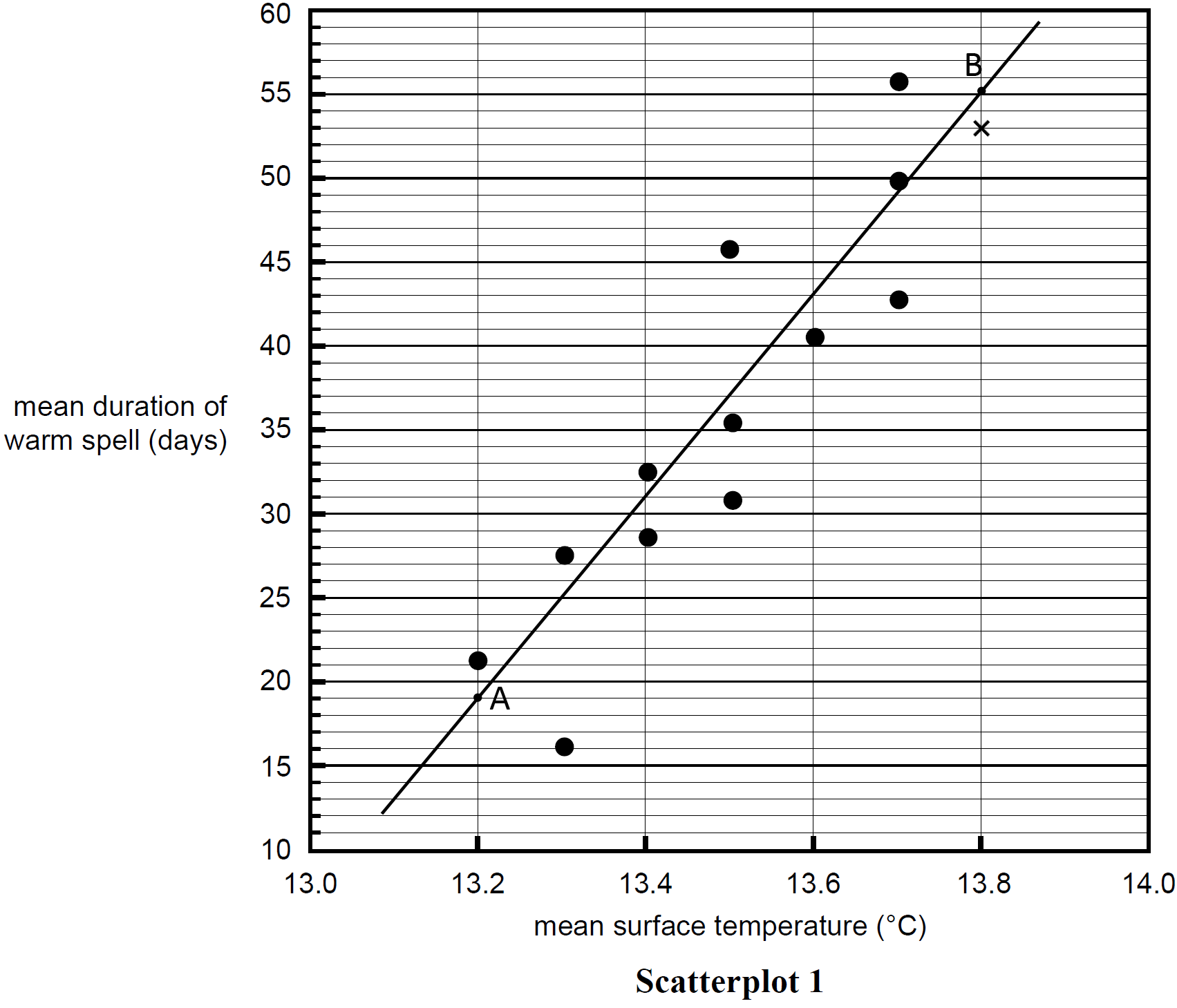
The table below displays the mean surface temperature (in °C) and the mean duration of warm spell (in days) in Australia for 13 years selected at random from the period 1960 to 2005.

This data set has been used to construct the scatterplot below. The scatterplot is incomplete.
- Complete the scatterplot below by plotting the bold data values given in the table above. Mark the point with a cross (×). (1 mark)
--- 0 WORK AREA LINES (style=lined) ---
- Mean surface temperature is the explanatory variable.
- Determine the equation of the least squares regression line for this set of data. Write the equation in terms of the variables mean duration of warm spell and mean surface temperature. Write the value of the coefficients correct to one decimal place. (2 marks)
--- 2 WORK AREA LINES (style=lined) ---
- Plot the least squares regression line on Scatterplot 1. (1 mark)
--- 0 WORK AREA LINES (style=lined) ---
- Determine the equation of the least squares regression line for this set of data. Write the equation in terms of the variables mean duration of warm spell and mean surface temperature. Write the value of the coefficients correct to one decimal place. (2 marks)

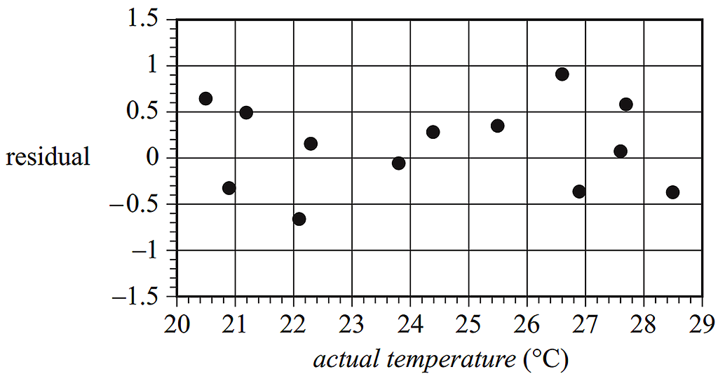
The residual plot below was constructed to test the assumption of linearity for the relationship between the variables mean duration of warm spell and the mean surface temperature.

- Explain why this residual plot supports the assumption of linearity for this relationship. (1 mark)
--- 1 WORK AREA LINES (style=lined) ---
- Write down the percentage of variation in the mean duration of a warm spell that is explained by the variation in mean surface temperature. Write your answer correct to the nearest per cent. (1 mark)
--- 1 WORK AREA LINES (style=lined) ---
- Describe the relationship between the mean duration of a warm spell and the mean surface temperature in terms of strength, direction and form. (2 marks)
--- 2 WORK AREA LINES (style=lined) ---
Show Answers Only
-
- `text{See part b.ii. below.}`
- `text(Mean duration of warm spell)`
`= -776.9 + 60.3 xx text(mean surface temperature)`
- `text(Linearity is supported because there is no)`
`text(pattern to the residual data.)` - `83text(%)`
- `text(Strong, positive, and linear.)`
Show Worked Solution
| a. |  |
b.i. `text(Mean duration of warm spell)`
`= -776.9 + 60.3 xx text(mean surface temperature)`
MARKER’S COMMENT: A consistent error in these type of questions is taking 2 points that are too close together!
b.ii. `text(Taking extreme points on the above graph,)`
`text(When)\ \ x = 13.2, \ y = -776.9 + 60.3 xx 13.2 = 19.06`
`:.\ text(Passes through)\ \ A (13.2, 19.06)`
`text(When)\ x = 13.8, y = -776.9 + 60.3 xx 13.8 = 55.24`
`:.\ text(Passes through)\ \ B (13.8, 55.24)`
`text(*See the regression line plotted above.)`
c. `text(Linearity is supported because there is no)`
`text(pattern to the residual data.)`
d. `text(By Calculator,)`
`r^2 = 0.828… = 83text{% (nearest %)}`
e. `text(Strong, positive, and linear.)`
CORE, FUR2 2008 VCAA 4
The arm spans (in cm) and heights (in cm) for a group of 13 boys have been measured. The results are displayed in the table below.

The aim is to find a linear equation that allows arm span to be predicted from height.
- What will be the explanatory variable in the equation? (1 mark)
--- 1 WORK AREA LINES (style=lined) ---
- Assuming a linear association, determine the equation of the least squares regression line that enables arm span to be predicted from height. Write this equation in terms of the variables arm span and height. Give the coefficients correct to two decimal places. (2 marks)
--- 2 WORK AREA LINES (style=lined) ---
- Using the equation that you have determined in part b., interpret the slope of the least squares regression line in terms of the variables height and arm span. (1 mark)
--- 2 WORK AREA LINES (style=lined) ---
CORE, FUR2 2015 VCAA 4
The table below shows male life expectancy (male) and female life expectancy (female) for a number of countries in 2013. The scatterplot has been constructed from this data.

- Use the scatterplot to describe the association between male life expectancy and female life expectancy in terms of strength, direction and form. (1 mark)
--- 3 WORK AREA LINES (style=lined) ---
- Determine the equation of a least squares regression line that can be used to predict male life expectancy from female life expectancy for the year 2013.
Complete the equation for the least squares regression line below by writing the intercept and slope in the space provided.
Write these values correct to two decimal places. (1 mark)
--- 0 WORK AREA LINES (style=lined) ---
male = ______________ + ______________ × female
CORE, FUR1 2015 VCAA 9 MC

A least squares regression line has been fitted to the scatterplot above to enable distance, in kilometres, to be predicted from time, in minutes.
The equation of this line is closest to
A. distance `= 3.5 + 1.6 ×`time
B. time `= 3.5 + 1.6 ×`distance
C. distance `= 1.6 + 3.5 ×`time
D. time `= 1.8 + 3.5 ×`distance
E. distance `= 3.5 + 1.8 ×`time
CORE, FUR1 2014 VCAA 9 MC
The equation of a least squares regression line is used to predict the fuel consumption, in kilometres per litre of fuel, from a car’s weight, in kilograms.
This equation predicts that a car weighing 900 kg will travel 10.7 km per litre of fuel, while a car weighing 1700 kg will travel 6.7 km per litre of fuel.
The slope of this least squares regression line is closest to
A. `–250`
B. `–0.005`
C. `–0.004`
D. `0.005`
E. `200`

CORE, FUR1 2011 VCAA 6-8 MC
When blood pressure is measured, both the systolic (or maximum) pressure and the diastolic (or minimum) pressure are recorded.
Table 1 displays the blood pressure readings, in mmHg, that result from fifteen successive measurements of the same person's blood pressure.

Part 1
Correct to one decimal place, the mean and standard deviation of this person's systolic blood pressure measurements are respectively
A. `124.9 and 4.4`
B. `125.0 and 5.8`
C. `125.0 and 6.0`
D. `125.9 and 5.8`
E. `125.9 and 6.0`
Part 2
Using systolic blood pressure (systolic) as the response variable, and diastolic blood pressure (diastolic) as the explanatory variable, a least squares regression line is fitted to the data in Table 1.
The equation of the least squares regression line is closest to
A. `text(systolic) = 70.3 + 0.790 xx text(diastolic)`
B. `text(diastolic) = 70.3 + 0.790 xx text(systolic)`
C. `text(systolic) = 29.3 + 0.330 xx text(diastolic)`
D. `text(diastolic) = 0.330 + 29.3 xx text(systolic)`
E. `text(systolic) = 0.790 + 70.3 xx text(diastolic)`
Part 3
From the fifteen blood pressure measurements for this person, it can be concluded that the percentage of the variation in systolic blood pressure that is explained by the variation in diastolic blood pressure is closest to
A. `25.8text(%)`
B. `50.8text(%)`
C. `55.4text(%)`
D. `71.9text(%)`
E. `79.0text(%)`
CORE, FUR1 2010 VCAA 7-9 MC
The height (in cm) and foot length (in cm) for each of eight Year 12 students were recorded and displayed in the scatterplot below.
A least squares regression line has been fitted to the data as shown.

Part 1
By inspection, the value of the product-moment correlation coefficient `(r)` for this data is closest to
- `0.98`
- `0.78`
- `0.23`
- `– 0.44`
- `– 0.67`
Part 2
The explanatory variable is foot length.
The equation of the least squares regression line is closest to
- height = –110 + 0.78 × foot length.
- height = 141 + 1.3 × foot length.
- height = 167 + 1.3 × foot length.
- height = 167 + 0.67 × foot length.
- foot length = 167 + 1.3 × height.
Part 3
The plot of the residuals against foot length is closest to


CORE, FUR1 2012 VCAA 8 MC
The maximum wind speed and maximum temperature were recorded each day for a month. The data is displayed in the scatterplot below and a least squares regression line has been fitted. The response variable is temperature. The explanatory variable is wind speed.

The equation of the least squares regression line is closest to
A. `text(temperature) = 25.7 - 0.191 xx text(wind speed)`
B. `text(wind speed) = 25.7 - 0.191 xx text(temperature)`
C. `text(temperature) = 0.191 + 25.7 xx text(wind speed)`
D. `text(wind speed) = 25.7 + 0.191 xx text(temperature)`
E. `text(temperature) = 25.7 + 0.191 xx text(wind speed)`
CORE, FUR1 2009 VCAA 9-10 MC
The table below lists the average life span (in years) and average sleeping time (in hours/day) of 12 animal species.

Part 1
Using sleeping time as the independent variable, a least squares regression line is fitted to the data.
The equation of the least squares regression line is closest to
A. life span = 38.9 – 2.36 × sleeping time.
B. life span = 11.7 – 0.185 × sleeping time.
C. life span = – 0.185 – 11.7 × sleeping time.
D. sleeping time = 11.7 – 0.185 × life span.
E. sleeping time = 38.9 – 2.36 × life span.
Part 2
The value of Pearson’s product-moment correlation coefficient for life span and sleeping time is closest to
A. `–0.6603`
B. `–0.4360`
C. `–0.1901`
D. `0.4360`
E. `0.6603`