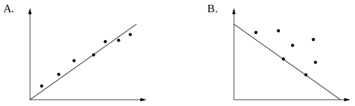
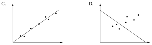
Each of the scatterplots shows the same number of data points.
Which scatterplot has the most appropriate line of best fit?
Aussie Maths & Science Teachers: Save your time with SmarterEd
Each of the scatterplots shows the same number of data points.
Which scatterplot has the most appropriate line of best fit?
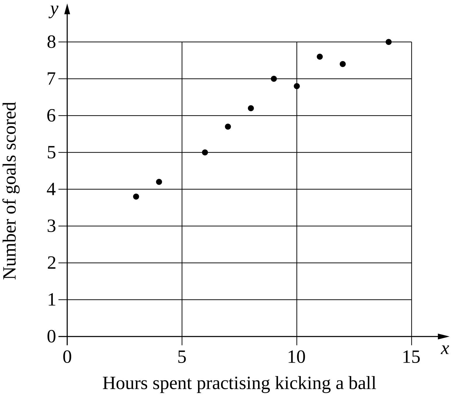
A coach was interested in whether there was a relationship between the number of hours spent practising kicking a ball and the number of goals scored in a competition.
The coach collected data from 10 players. A graph of the dataset is shown.
--- 0 WORK AREA LINES (style=lined) ---
--- 2 WORK AREA LINES (style=lined) ---
A researcher is using the statistical investigation process to investigate a possible relationship between average number of minutes per day a person spends watching television, and the average number of minutes per day the person spends exercising.
--- 3 WORK AREA LINES (style=lined) ---
Participants were asked to record the number of minutes they spent watching television each day and the number of minutes they spent exercising each day. The averages for each participant were recorded and graphed, and a line of best fit was included.

--- 1 WORK AREA LINES (style=lined) ---
--- 3 WORK AREA LINES (style=lined) ---
--- 10 WORK AREA LINES (style=lined) ---
--- 4 WORK AREA LINES (style=lined) ---
a. \(\text{How does the average daily time spent watching television}\)
\(\text{relate to the average daily time spent exercising?}\)
b. \(\text{Dependent variable:}\)
\(\text{Average minutes per day exercising, or }y.\)
c. \(\text{Form: Linear}\)
\(\text{Direction: Negative}\)

\(y-\text{intercept = 70}\)
\(\text{Gradient}=\dfrac{\text{rise}}{\text{run}}=\dfrac{-60}{60}=-1\)
e. \(\text{The extrapolation of the graph past 70 minutes produces}\)
\(\text{negative average minutes per day exercising (impossible).}\)
The scatterplot shows the number of ice-creams sold, \(y\), at a shop over a ten-day period, and the temperature recorded at 2 pm on each of these days. \(y=0.936 x-8.929\), where \(x\) is the temperature. --- 4 WORK AREA LINES (style=lined) --- --- 3 WORK AREA LINES (style=lined) ---

A teacher surveyed the students in her Year 8 class to investigate the relationship between the average number of hours of phone use per day and the average number of hours of sleep per day.
The results are shown on the scatterplot below.

\begin{array} {|l|c|c|}
\hline
& \textit{Average hours of} & \textit{Average hours of} \\ & \textit{phone use per day} & \textit{sleep per day} \\
\hline
\rule{0pt}{2.5ex} \text{Alinta} \rule[-1ex]{0pt}{0pt} & 4 & 8 \\
\hline
\rule{0pt}{2.5ex} \text{Birrani} \rule[-1ex]{0pt}{0pt} & 0 & 10.5 \\
\hline
\end{array}
--- 2 WORK AREA LINES (style=lined) ---
a.

b. \(\text{9 hours of sleep per day}\)
a.
b. \(\text{Using the line of best fit added to the diagram in part (a):}\)
\(\text{2 hours of phone use per day}\ \ \Rightarrow\ \ \text{9 hours of sleep per day}\)
A concert organiser is interested in the relationship between the distance from the stage, in metres, and the loudness of the sound measured in decibels.
The data the concert organiser collected is shown on the graph.

--- 1 WORK AREA LINES (style=lined) ---
--- 1 WORK AREA LINES (style=lined) ---
People are placed into groups to complete a puzzle. There are 9 different groups.
The table shows the number of people in each group and the amount of time, in minutes, for each group to complete the puzzle.
\begin{array} {|l|c|c|c|c|c|c|c|c|c|}
\hline
\rule{0pt}{2.5ex} \textit{Number of people} \rule[-1ex]{0pt}{0pt} & 2 & 2 & 3 & 5 & 5 & 7 & 7 & 7 & 8 \\
\hline
\rule{0pt}{2.5ex} \textit{Time taken (min)} \rule[-1ex]{0pt}{0pt} & 28 & 30 & 26 & 19 & 21 & 12 & 13 & 11 & 8 \\
\hline
\end{array}

--- 3 WORK AREA LINES (style=lined) ---
--- 1 WORK AREA LINES (style=lined) ---
a.

b.

c. `text(The association is linear, negative and strong.)`
d. `12\ text(minutes)`
a.
b.
c. `text(Form: linear)`
`text{Direction: negative}`
`text{Strength: strong}`
d. `text{Mean time (7 people)}= (12 + 13 + 11)/3= 12\ text(minutes)`
A group of students sat a test at the end of term. The number of lessons each student missed during the term and their score on the test are shown on the scatterplot.

--- 5 WORK AREA LINES (style=lined) ---
--- 1 WORK AREA LINES (style=lined) ---
Use the line of the best fit drawn in part (c) to estimate Meg's score on this test. (1 mark)
--- 1 WORK AREA LINES (style=lined) ---
Is it appropriate to use the line of the best fit to estimate his score on the test? Briefly explain your answer. (1 mark)
--- 2 WORK AREA LINES (style=lined) ---
a. \(\text{Strength : strong}\)
\(\text{Direction : negative} \)
b. \(\text{Range}\ = \text{high}-\text{low}\ = 100-80=20\)
c.

d.

e. \(\text{John’s missed days are too extreme and the LOBF is not}\)
\(\text{appropriate. The model would estimate a negative score for}\)
\(\text{John which is impossible.}\)
a. \(\text{Strength : strong}\)
\(\text{Direction : negative} \)
b. \(\text{Range}\ = \text{high}-\text{low}\ = 100-80=20\)
c.
d.
\(\therefore\ \text{Meg’s estimated score = 40}\)
e. \(\text{John’s missed days are too extreme and the LOBF is not}\)
\(\text{appropriate. The model would estimate a negative score for}\)
\(\text{John which is impossible.}\)
A set of bivariate data is collected by measuring the height and arm span of eight children. The graph shows a scatterplot of these measurements.

--- 0 WORK AREA LINES (style=lined) ---
--- 1 WORK AREA LINES (style=lined) ---
a.

b. `text(Robert’s height ≈ 151.1 cm)`
a.
b. `text(Robert’s height ≈ 151.1 cm)`
`text{(Answers can vary slightly depending on line of best fit drawn).}`
The graph shows the relationship between infant mortality rate (deaths per 1000 live births) and life expectancy at birth (in years) for different countries.

What is the life expectancy at birth in a country which has an infant mortality rate of 60?
\(\text{When infant mortality rate is 60, life expectancy}\)
\(\text{at birth is 68 years (see below).}\)

\(\Rightarrow A\)