SmarterEd

Aussie Maths & Science Teachers: Save your time with SmarterEd

  • Login
  • Get Help
  • About

Statistical, STD2 EQ-Bank 30

A teacher surveyed the students in her Year 8 class to investigate the relationship between the number of hours of phone use per day and the number of hours of sleep per day.

The results for five students are shown on the scatterplot. The least-squares regression line is also shown.
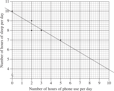


  1. Calculate Pearson's correlation coefficient \((r)\), to 4 decimal places, and describe the relationship between number of hours of sleep per day and number of hours of phone use per day.   (3  marks)

    --- 4 WORK AREA LINES (style=lined) ---

  2. Find the equation of the least-squares regression line.   (2  marks)

    --- 2 WORK AREA LINES (style=lined) ---

  3. From the data, the median number of hours of phone use per day, \(a\), and the median of the number of hours of sleep per day, \(b\), are to be calculated.
  4. By finding the coordinates \((a, b)\), determine whether this point would lie on, below or above the least-squares regression line.   (3  marks)

    --- 3 WORK AREA LINES (style=lined) ---
Show Answers Only

a.    \(r=-0.9414\)

\(\text{There is a strong, negative linear relationship between number of hours of sleep}\)

\(\text{per day and number of hours of phone use per day.}\)
 

b.    \(\text{By calculator (inputting all data points):}\)

\(y=-0.591 x+9.818 \ \text{(3 d.p.)}\)
 

c.    \(x\text{-values of data points:}\ {0,2,2,3,5}\)

\(\text{Median of the number of hours of phone use = 2 hours}\)

\(y\text{-values of data points:}\ {7,8,8,9,10}\)

\(\text{Median of the number of hours of sleep = 8 hours}\)

\((a,b) = (2,8)\ \ \Rightarrow\ \ \text{this point lies below the LSRL.}\)

Show Worked Solution

a.    \(r=-0.9414\)

\(\text{There is a strong, negative linear relationship between number of hours of sleep}\)

\(\text{per day and number of hours of phone use per day.}\)
 

b.    \(\text{By calculator (inputting all data points):}\)

\(y=-0.591 x+9.818 \ \text{(3 d.p.)}\)
 

c.    \(x\text{-values of data points:}\ {0,2,2,3,5}\)

\(\text{Median of the number of hours of phone use = 2 hours}\)

\(y\text{-values of data points:}\ {7,8,8,9,10}\)

\(\text{Median of the number of hours of sleep = 8 hours}\)

\((a,b) = (2,8)\ \ \Rightarrow\ \ \text{this point lies below the LSRL.}\)

Filed Under: Bivariate Data Analysis (Y12) Tagged With: Band 4, Band 5, smc-6934-20-LSRL, smc-6934-40-Pearson’s

Statistics, STD2 S4 2023 HSC 3 MC

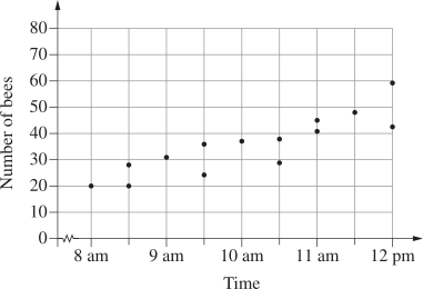
The number of bees leaving a hive was observed and recorded over 14 days at different times of the day.
 

Which Pearson's correlation coefficient best describes the observations?

  1. `-0.8`
  2. `-0.2`
  3. `0.2`
  4. `0.8`
Show Answers Only

`D`

Show Worked Solution

`text{Correlation is positive and strong.}`

`text{Best option:}\ r=0.8`

`=>D`

NOTE: Inputting all data points into a calculator is unnecessary and time consuming here.

Filed Under: Bivariate Data Analysis (Y12), S4 Bivariate Data Analysis (Y12) Tagged With: 2adv-std2-common, Band 4, common-content, smc-6934-40-Pearson’s, smc-6934-70-Calculator (Stats Mode), smc-785-40-Pearson's, smc-785-70-Calculator (Stats Mode)

Statistics, STD2 S4 2020 HSC 12 MC

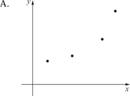
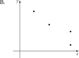
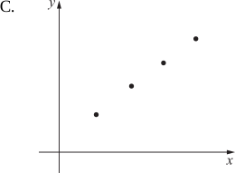
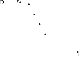
For a set of bivariate data, Pearson's correlation coefficient is  –1.

Which graph could best represent this set of bivariate data?


Show Answers Only

`D`

Show Worked Solution

`text(Negative correlation coefficient:)`

`text(Line of Best Fit will go from top left to bottom right)`

`text(Correlation coefficient of magnitude 1:)`

`text(Data will be in a straight line.)`

`=> D`

Filed Under: Bivariate Data Analysis (Y12), S4 Bivariate Data Analysis (Y12) Tagged With: Band 4, common-content, smc-6934-40-Pearson’s, smc-785-40-Pearson's

Statistics, STD2 S4 EQ-Bank 26

Ten high school students have their height and the length of their right foot measured.

The results are recorded in the table below.


  1. Using technology, calculate Pearson's correlation coefficient for the data. Give your answer to 3 decimal places.   (1 mark)

    --- 1 WORK AREA LINES (style=lined) ---

  2. Describe the strength of the association between height and length of right foot for these students.   (1 mark)

    --- 2 WORK AREA LINES (style=lined) ---
  3. Using technology, determine the least squares regression line that allows height to be predicted from right foot length.   (1 mark)

    --- 1 WORK AREA LINES (style=lined) ---

Show Answers Only

a.    `0.941\ \ (text(to 3 d.p.))`

b.    `text(The association is positive and strong.)`

c.    `text(Height) =47.4 + 4.7 xx text(foot length)`

Show Worked Solution

a.    `text(By calculator,)`

COMMENT: Issues here? YouTube has short and excellent help videos – search your calculator model and topic – eg. “fx-82 correlation” .

`r` `= 0.94095…`
  `= 0.941\ \ (text(to 3 d.p.))`

  
b.
    `text(The association is positive and strong.)`
  

c.    `x\ text(value ⇒ foot length (independent variables))`

`y\ text(value ⇒ height.)`

`text(By calculator:)`

`text(Height) = 47.4 + 4.7 xx text(foot length)`

Filed Under: Bivariate Data Analysis, Bivariate Data Analysis (Y12), S4 Bivariate Data Analysis (Y12) Tagged With: Band 4, common-content, smc-1001-20-Least-Squares Regression Line, smc-1001-30-Correlation, smc-1001-40-Pearson's, smc-1001-70-Calculator (Stats Mode), smc-6934-20-LSRL, smc-6934-30-Correlation, smc-6934-40-Pearson’s, smc-6934-70-Calculator (Stats Mode), smc-785-20-Least-Squares Regression Line, smc-785-30-Correlation, smc-785-40-Pearson's, smc-785-70-Calculator (Stats Mode)

Statistics, STD2 S4 2019 HSC 23

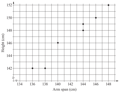
A set of bivariate data is collected by measuring the height and arm span of seven children. The graph shows a scatterplot of these measurements.


  1. Calculate Pearson's correlation coefficient for the data, correct to two decimal places.   (1 mark)

    --- 1 WORK AREA LINES (style=lined) ---

  2. Identify the direction and the strength of the linear association between height and arm span.   (1 mark)

    --- 2 WORK AREA LINES (style=lined) ---

  3. The equation of the least-squares regression line is shown.
     
               Height = 0.866 × (arm span) + 23.7
     
    A child has an arm span of 143 cm.


    Calculate the predicted height for this child using the equation of the least-squares regression line.   (1 mark)

    --- 1 WORK AREA LINES (style=lined) ---

Show Answers Only

a.    `0.98\ \ (text(2 d.p.))`

b.    `text(Direction: positive)`

`text(Strength: strong)`

c.    `147.538\ text(cm)`

Show Worked Solution

a.    `text{Use  “A + Bx”  function (fx-82 calc):}`

♦ Mean mark 40%.
COMMENT: Issues here? YouTube has short and excellent help videos – search your calculator model and topic – eg. “fx-82 correlation” .

`r` `= 0.9811…`
  `= 0.98\ \ (text(2 d.p.))`

  
b.
    `text(Direction: positive)`

`text(Strength: strong)`
  

c.     `text(Height)` `= 0.866 xx 143 + 23.7`
    `= 147.538\ text(cm)`

Filed Under: Bivariate Data Analysis, Bivariate Data Analysis (Y12), S4 Bivariate Data Analysis (Y12) Tagged With: Band 3, Band 4, Band 5, common-content, smc-1001-30-Correlation, smc-1001-40-Pearson's, smc-1001-70-Calculator (Stats Mode), smc-6934-30-Correlation, smc-6934-40-Pearson’s, smc-6934-70-Calculator (Stats Mode), smc-785-30-Correlation, smc-785-40-Pearson's, smc-785-70-Calculator (Stats Mode)

Copyright © 2014–2026 SmarterEd.com.au · Log in