SmarterEd

Aussie Maths & Science Teachers: Save your time with SmarterEd

  • Login
  • Get Help
  • About

Statistical, STD2 EQ-Bank 30

A teacher surveyed the students in her Year 8 class to investigate the relationship between the number of hours of phone use per day and the number of hours of sleep per day.

The results for five students are shown on the scatterplot. The least-squares regression line is also shown.
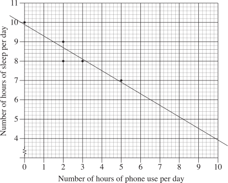


  1. Calculate Pearson's correlation coefficient \((r)\), to 4 decimal places, and describe the relationship between number of hours of sleep per day and number of hours of phone use per day.   (3  marks)

    --- 4 WORK AREA LINES (style=lined) ---

  2. Find the equation of the least-squares regression line.   (2  marks)

    --- 2 WORK AREA LINES (style=lined) ---

  3. From the data, the median number of hours of phone use per day, \(a\), and the median of the number of hours of sleep per day, \(b\), are to be calculated.
  4. By finding the coordinates \((a, b)\), determine whether this point would lie on, below or above the least-squares regression line.   (3  marks)

    --- 3 WORK AREA LINES (style=lined) ---
Show Answers Only

a.    \(r=-0.9414\)

\(\text{There is a strong, negative linear relationship between number of hours of sleep}\)

\(\text{per day and number of hours of phone use per day.}\)
 

b.    \(\text{By calculator (inputting all data points):}\)

\(y=-0.591 x+9.818 \ \text{(3 d.p.)}\)
 

c.    \(x\text{-values of data points:}\ {0,2,2,3,5}\)

\(\text{Median of the number of hours of phone use = 2 hours}\)

\(y\text{-values of data points:}\ {7,8,8,9,10}\)

\(\text{Median of the number of hours of sleep = 8 hours}\)

\((a,b) = (2,8)\ \ \Rightarrow\ \ \text{this point lies below the LSRL.}\)

Show Worked Solution

a.    \(r=-0.9414\)

\(\text{There is a strong, negative linear relationship between number of hours of sleep}\)

\(\text{per day and number of hours of phone use per day.}\)
 

b.    \(\text{By calculator (inputting all data points):}\)

\(y=-0.591 x+9.818 \ \text{(3 d.p.)}\)
 

c.    \(x\text{-values of data points:}\ {0,2,2,3,5}\)

\(\text{Median of the number of hours of phone use = 2 hours}\)

\(y\text{-values of data points:}\ {7,8,8,9,10}\)

\(\text{Median of the number of hours of sleep = 8 hours}\)

\((a,b) = (2,8)\ \ \Rightarrow\ \ \text{this point lies below the LSRL.}\)

Filed Under: Bivariate Data Analysis (Y12) Tagged With: Band 4, Band 5, smc-6934-20-LSRL, smc-6934-40-Pearson’s

Statistics, STD2 EQ-Bank 29

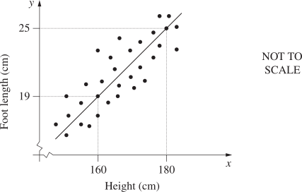
Each member of a group of males had his height and foot length measured and recorded. The results were graphed and a line of fit drawn.
 

  1. Identify the independent variable.   (1 mark)

    --- 1 WORK AREA LINES (style=lined) ---

  2. Why does the value of the `y`-intercept have no meaning in this situation?   (1 mark)

    --- 2 WORK AREA LINES (style=lined) ---

  3. George is 10 cm taller than his brother Harry. Use the line of fit to estimate the difference in their foot lengths.   (1 mark)

    --- 2 WORK AREA LINES (style=lined) ---

Show Answers Only

a.    `text{Height is the independent variable (x-axis variable).}`
 

b.    `text(The y-intercept occurs when)\ x = 0.\ text(It has no meaning to have)`

`text(a height of 0 cm.)`
  

c.    `text(A 20 cm height difference results in a foot length difference of 6 cm.)`

`text(A 10 cm height difference means George should have a 3 cm longer foot.)`

Show Worked Solution

a.    `text{Height is the independent variable (x-axis variable).}`
 

b.    `text(The y-intercept occurs when)\ x = 0.\ text(It has no meaning to have)`

`text(a height of 0 cm.)`
  

c.    `text(A 20 cm height difference results in a foot length difference of 6 cm.)`

`text(A 10 cm height difference means George should have a 3 cm longer foot.)`

Filed Under: Bivariate Data Analysis (Y12) Tagged With: Band 3, Band 4, Band 5, smc-6934-10-Line of Best Fit

Statistics, STD2 S4 2025 HSC 25

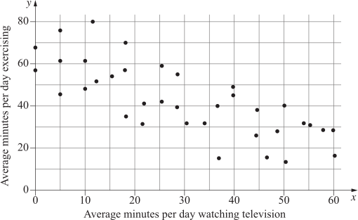
In a research study, participants were asked to record the number of minutes they spent watching television and the number of minutes they spent exercising each day over a period of 3 months. The averages for each participant were recorded and graphed.
 

  1. Describe the bivariate dataset in terms of its form and direction.   (2 marks)
  2. Form:  ..................................................................
  3. Direction:  ............................................................

    --- 0 WORK AREA LINES (style=lined) ---

The equation of the least-squares regression line for this dataset is

\(y=64.3-0.7 x\)

  1. Interpret the values of the slope and \(y\)-intercept of the regression line in the context of this dataset.   (2 marks)

    --- 6 WORK AREA LINES (style=lined) ---

  2. Jo spends an average of 42 minutes per day watching television.
  3. Use the equation of the regression line to determine how many minutes on average Jo is expected to exercise each day.   (1 mark)

    --- 4 WORK AREA LINES (style=lined) ---

  4. Explain why it is NOT appropriate to extrapolate the regression line to predict the average number of minutes of exercise per day for someone who watches an average of 2 hours of television per day.   (1 mark)

    --- 4 WORK AREA LINES (style=lined) ---

Show Answers Only

a.    \(\text{Form: Linear. Direction: Negative}\)

b.    \(\text{Slope}=-0.7\)

This means that for each added minute of watching television per day, a participant, on average, will exercise for 0.7 minutes less.

\(y \text{-intercept}=64.3\)

If someone watches no television, the LSRL predicts they will exercise for 64.3 minutes per day.

c.    Jo is expected to exercise for 34.9 minutes.

d.    \(\text{At} \ \  x=120\ \text{(2 hours),} \ \ y=64.3-0.7 \times 120=-19.7\)

The model predicts a negative value for time spent exercising, which is not possible.

Show Worked Solution

a.    Form: Linear

Direction: Negative

Mean mark (a) 51%.

b.    \(\text{Slope}=-0.7\)

This means that for each added minute of watching television per day, a participant, on average, will exercise for 0.7 minutes less.

\(y \text{-intercept}=64.3\)

If someone watches no television, the LSRL predicts they will exercise for 64.3 minutes per day.

♦♦♦ Mean mark (b) 20%.

c.    \(\text{At} \ \ x=42:\)

\(y=64.3-0.7 \times 42=34.9\)

\(\therefore\) Jo is expected to exercise for 34.9 minutes.
 

d.    \(\text{At} \ \  x=120\ \text{(2 hours),} \ \ y=64.3-0.7 \times 120=-19.7\)

The model predicts a negative value for time spent exercising, which is not possible.

♦ Mean mark (d) 45%.

Filed Under: Bivariate Data Analysis (Y12), S4 Bivariate Data Analysis (Y12) Tagged With: 2adv-std2-common, Band 4, Band 5, Band 6, smc-6934-20-LSRL, smc-6934-50-Gradient Interpretation, smc-6934-60-Limitations, smc-785-20-Least-Squares Regression Line, smc-785-50-Gradient Interpretation, smc-785-60-Limitations

Statistics, STD2 S4 2025 HSC 17

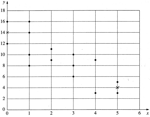
The scatter plot shows a bivariate dataset, where \(x\) is the independent variable and \(y\) is the dependent variable. 


The points \( (0,14) \) and \( (5,4)\) lie on the line of best fit.

Plot the points \( (0,14) \) and \( (5,4) \) on the graph and hence find the equation of the line of best fit.   (3 marks)

--- 6 WORK AREA LINES (style=lined) ---

Show Answers Only

\( y=-2 x+14 \)

Show Worked Solution

\(\text{Gradient (LOBF)}\ =\dfrac{y_2-y_1}{x_4-x_1}=\dfrac{4-14}{5-0}=-2 \)

\(\text{Find equation of line}\ \ m=-2 \ \ \text{through}\ (0,14):\)

\( y-y_1\) \(=m(x-x_1)\)
\( y-14\) \(=-2(x-0)\)
\( y\) \(=-2 x+14 \)

Filed Under: Bivariate Data Analysis (Y12), S4 Bivariate Data Analysis (Y12) Tagged With: Band 4, smc-6934-10-Line of Best Fit, smc-785-10-Line of Best Fit

Statistics, STD2 S4 2024 HSC 19

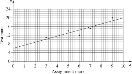
A teacher was exploring the relationship between students' marks for an assignment and their marks for a test. The data for five different students are shown on the graph.

The least-squares regression line is also shown.
 

  1. What is the equation of the least-squares regression line for this dataset?   (2 marks)

    --- 4 WORK AREA LINES (style=lined) ---

  2. Another student, whose marks are not on the graph, scored 5 for the assignment and 12 on the test.
  3. Did this student do better or worse on the test than the regression line predicts? Provide a reason for your answer.   (1 mark)

    --- 4 WORK AREA LINES (style=lined) ---

Show Answers Only

a.    \(\text {Data points: }(3,11),(5,14),(6,12),(7,15),(9,20)\)

\(y \,\text {-intercept}=6\)

\(m=\dfrac{y_2-y_1}{x_2-x_1}=\dfrac{20-6}{10-0}=1.4\)

\(\text{LSRL}\ \ \Rightarrow \ y=1.4x+6\)
 

b.    \(\text {The student’s mark \((5,12)\) sits below the LSRL.}\)

 \(\text {Therefore the student did worse than expected.}\)

Show Worked Solution

a.    \(\text {Data points: }(3,11),(5,14),(6,12),(7,15),(9,20)\)

\(y\,\text {-intercept}=6\)

\(m=\dfrac{y_2-y_1}{x_2-x_1}=\dfrac{20-6}{10-0}=1.4\)

\(\text{LSRL}\ \ \Rightarrow \ y=1.4x+6\)

♦ Mean mark (a) 46%.

b.    \(\text {The student’s mark \((5,12)\) sits below the LSRL.}\)

 \(\text {Therefore the student did worse than expected.}\)

Filed Under: Bivariate Data Analysis (Y12), S4 Bivariate Data Analysis (Y12) Tagged With: Band 4, Band 5, smc-6934-20-LSRL, smc-785-20-Least-Squares Regression Line

Statistics, STD2 S4 2024 HSC 30

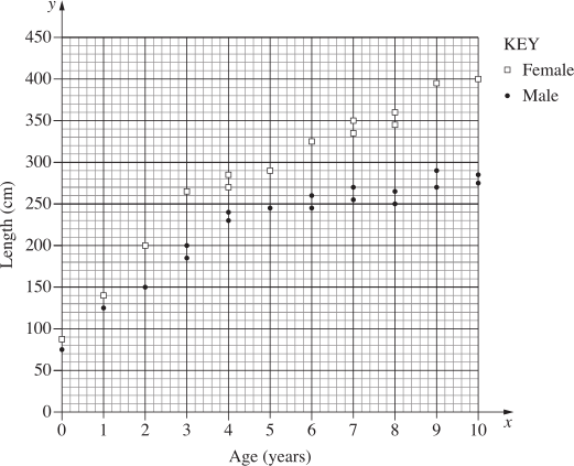
A researcher is studying anacondas (a type of snake).

A dataset recording the age (in years) and length (in cm) of female and male anacondas is displayed on the graph.

Anacondas reach maturity at about 4 years of age.
 

Write THREE observations about anacondas that may be made from the scatterplot. (Note: No calculations are required.)   (3 marks)

--- 6 WORK AREA LINES (style=lined) ---

Show Answers Only

\(\text{Answers could include three of the following:}\)

\(\rightarrow\ \text{Female anacondas are longer than males of the equivalent age.}\)

\(\rightarrow\ \text{Female anacondas grow more quickly than male anacondas from birth until}\)

\(\text{maturity which can be seen by the steeper gradient of the LOBF for each dataset}\)

\(\text{over this period.}\)

\(\rightarrow\ \text{Female anacondas continue to grow to at least 10 years of age, well past their}\)

\(\text{age of maturity at 4 years of age.}\)

\(\rightarrow\ \text{Male anacondas’ growth slows noticeably and flattens out once they hit their}\)

\(\text{age of maturity at 4 years old.}\)

Show Worked Solution

\(\text{Answers could include three of the following:}\)

\(\rightarrow\ \text{Female anacondas are longer than males of the equivalent age.}\)

\(\rightarrow\ \text{Female anacondas grow more quickly than male anacondas from birth until}\)

\(\text{maturity which can be seen by the steeper gradient of the LOBF for each dataset}\)

\(\text{over this period.}\)

\(\rightarrow\ \text{Female anacondas continue to grow to at least 10 years of age, well past their}\)

\(\text{age of maturity at 4 years of age.}\)

\(\rightarrow\ \text{Male anacondas’ growth slows noticeably and flattens out once they hit their}\)

\(\text{age of maturity at 4 years old.}\)

Filed Under: Bivariate Data Analysis (Y12), S4 Bivariate Data Analysis (Y12) Tagged With: 2adv-std2-common, Band 4, smc-6934-50-Gradient Interpretation, smc-6934-90-Data observations, smc-785-50-Gradient Interpretation, smc-785-90-Data observations

Statistics, STD2 S4 2023 HSC 34

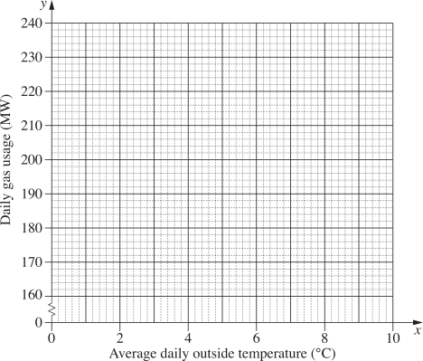
A university uses gas to heat its buildings. Over a period of 10 weekdays during winter, the gas used each day was measured in megawatts (MW) and the average outside temperature each day was recorded in degrees Celsius (°C).

Using `x` as the average daily outside temperature and `y` as the total daily gas usage, the equation of the least-squares regression line was found.

The equation of the regression line predicts that when the temperature is 0°C, the daily gas usage is 236 MW.

The ten temperatures measured were: 0°, 0°, 0°, 2°, 5°, 7°, 8°, 9°, 9°, 10°,

The total gas usage for the ten weekdays was 1840 MW.

In any bivariate dataset, the least-squares regression line passes through the point `(bar x,bar y)`, where `bar x` is the sample mean of the `x`-values and `bar y` is the sample mean of the `y`-values.

  1. Using the information provided, plot the point `(bar x,bar y)` and the `y`-intercept of the least-squares regression line on the grid.   (3 marks)

    --- 3 WORK AREA LINES (style=lined) ---


  1. What is the equation of the regression line?   (2 marks)

    --- 4 WORK AREA LINES (style=lined) ---
  2. In the context of the dataset, identify ONE problem with using the regression line to predict gas usage when the average outside temperature is 23°C.   (1 mark)

    --- 2 WORK AREA LINES (style=lined) ---
Show Answers Only

a.    
         

b.    `y=-10.4x+236`

c.    `text{Answers could include one of the following:}`

`text{→ 23°C is outside the range of the dataset and requires the trend}`

`text{to be extrapolated.}`

`text{→ At 23°C, the equation predicts negative daily gas usage.}`

Show Worked Solution

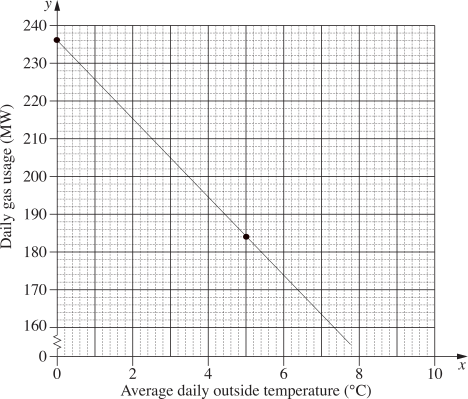
a.    `barx=(0+0+0+2+5+7+8+9+9+10)/10=5^@text{C}`

`bary=1840/10=184`

`text{Regression line passes through:}\ (0,236) and (5,184)`
 

♦ Mean mark (a) 44%.

b.    `m=(y_2-y_1)/(x_2-x_1)=(184-236)/(5-0)=-10.4`

`text{Equation of line}\ m=-10.4\ text{passing through}\ (0,236):`

`(y-y_1)` `=m(x-x_1)`
`y-236` `=-10.4(x-0)`
`y` `=-10.4x+236`
♦♦♦ Mean mark (b) 21%.

 c.    `text{Answers could include one of the following:}`

`text{→ 23°C is outside the range of the dataset and requires the trend}`

`text{to be extrapolated.}`

`text{→ At 23°C, the equation predicts negative daily gas usage.}`


♦♦ Mean mark (c) 23%.

Filed Under: Bivariate Data Analysis (Y12), S4 Bivariate Data Analysis (Y12) Tagged With: 2adv-std2-common, Band 5, Band 6, smc-6934-20-LSRL, smc-785-20-Least-Squares Regression Line

Statistics, STD2 S4 2023 HSC 3 MC

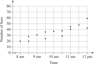
The number of bees leaving a hive was observed and recorded over 14 days at different times of the day.
 

Which Pearson's correlation coefficient best describes the observations?

  1. `-0.8`
  2. `-0.2`
  3. `0.2`
  4. `0.8`
Show Answers Only

`D`

Show Worked Solution

`text{Correlation is positive and strong.}`

`text{Best option:}\ r=0.8`

`=>D`

NOTE: Inputting all data points into a calculator is unnecessary and time consuming here.

Filed Under: Bivariate Data Analysis (Y12), S4 Bivariate Data Analysis (Y12) Tagged With: 2adv-std2-common, Band 4, common-content, smc-6934-40-Pearson’s, smc-6934-70-Calculator (Stats Mode), smc-785-40-Pearson's, smc-785-70-Calculator (Stats Mode)

Statistics, STD2 S4 2022 HSC 35

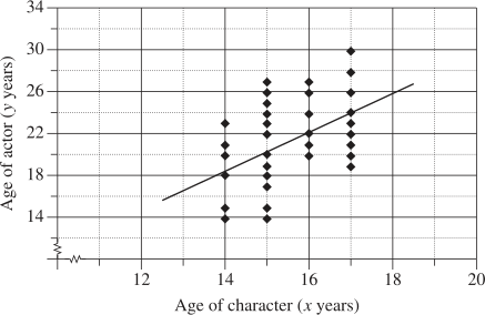
Jo is researching the relationship between the ages of teenage characters in television series and the ages of actors playing these characters.

After collecting the data, Jo finds that the correlation coefficient is 0.4564.

A scatterplot showing the data is drawn. The line of best fit with equation  `y=-7.51+1.85 x`, is also drawn.


Describe and interpret the data and other information provided, with reference to the context given.   (4 marks)

--- 8 WORK AREA LINES (style=lined) ---
Show Answers Only

`text{Correlation coefficient}\ (r) = 0.4564`

      • `text{Moderate and positive correlation}`

`text{Gradient of LOBF}\ = 1.85`

      • `text{On average, each extra year of a character’s age results}`
        `text{in the actor being 1.85 years older.}`

`text{Mode of data set = 15 years}`
  

`text{Limitations}`

      • `text{Data set is very restricted with just a 4 year range of}`
        `text{character ages.}`
      • `text{LOBF not useful when extrapolated to the left as it drops}`
        `text{below zero (on y-axis).}`
      • `text{Relationship describes correlation only, not causation.}`
Show Worked Solution

`text{Correlation coefficient}\ (r) = 0.4564`

      • `text{Moderate and positive correlation}`

`text{Gradient of LOBF}\ = 1.85`

      • `text{On average, each extra year of a character’s age results}`
        `text{in the actor being 1.85 years older.}`

`text{Mode of data set = 15 years}`
  

`text{Limitations}`

      • `text{Data set is very restricted with just a 4 year range of}`
        `text{character ages.}`
      • `text{LOBF not useful when extrapolated to the left as it drops}`
        `text{below zero (on y-axis).}`
      • `text{Relationship describes correlation only, not causation.}`

♦♦ Mean mark 30%.

Filed Under: Bivariate Data Analysis (Y12), S4 Bivariate Data Analysis (Y12) Tagged With: 2adv-std2-common, Band 5, common-content, smc-6934-30-Correlation, smc-6934-50-Gradient Interpretation, smc-6934-60-Limitations, smc-785-30-Correlation, smc-785-50-Gradient Interpretation, smc-785-60-Limitations

Statistics, STD2 S4 2022 HSC 23

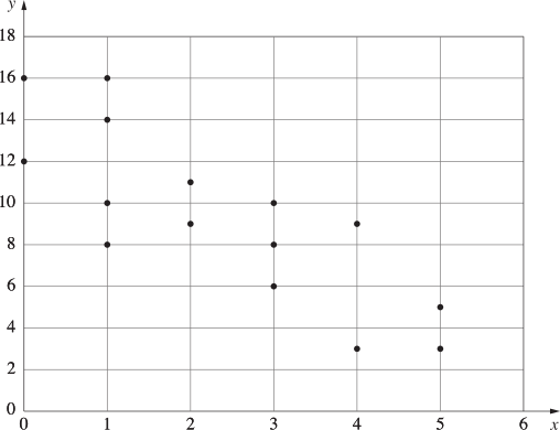
A teacher surveyed the students in her Year 8 class to investigate the relationship between the average number of hours of phone use per day and the average number of hours of sleep per day.

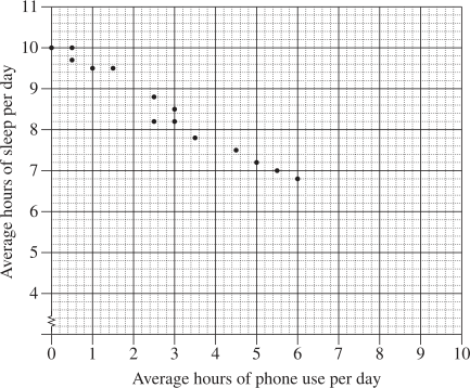
The results are shown on the scatterplot below.
 

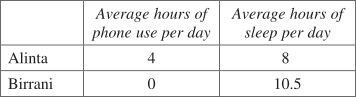
  1. The data for two new students, Alinta and Birrani, are shown in the table below. Plot their results on the scatterplot.   (2 marks)

    --- 0 WORK AREA LINES (style=lined) ---


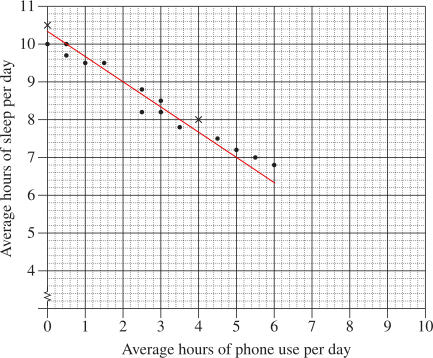
  2. By first fitting the line of best fit by eye on the scatterplot, estimate the average number of hours of sleep per day for a student who uses the phone for an average of 2 hours per day.   (2 marks)

    --- 4 WORK AREA LINES (style=lined) ---
Show Answers Only

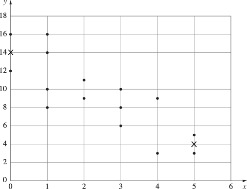
a.

b.    `text{9 hours (see LOBF in diagram above)}`

Show Worked Solution

a.   

b.    `text{9 hours (see LOBF in diagram above)}`

Filed Under: Bivariate Data Analysis (Y12), S4 Bivariate Data Analysis (Y12) Tagged With: Band 3, common-content, smc-6934-10-Line of Best Fit, smc-785-10-Line of Best Fit

Statistics, STD2 S4 2022 HSC 12 MC

For a particular course, the recorded data show a relationship between the number of hours of study per week and the marks achieved out of 100 .

A least-squares regression line is fitted to this dataset. The equation of this line is given by

`M=20+3 H,`

where `M` is the predicted mark and `H` is the number of hours of study per week.

Based on this regression equation, which of the following is correct regarding the predicted mark of a student?

  1. It will be 3 for zero hours of study per week.
  2. It will be 20 for zero hours of study per week.
  3. It will increase by 20 for every additional hour of study per week.
  4. It will increase by 1 for every 3 additional hours of study per week.
Show Answers Only

`B`

Show Worked Solution

`text{Consider Option}\ B:`

`text{If zero hours of study are done per week}\ \ → \ \ H=0`

`:. M=20+(3 xx 0) = 20`

`=>B`

Filed Under: Bivariate Data Analysis (Y12), S4 Bivariate Data Analysis (Y12) Tagged With: Band 4, common-content, smc-6934-50-Gradient Interpretation, smc-785-50-Gradient Interpretation

Statistics, STD2 S4 2021 HSC 33

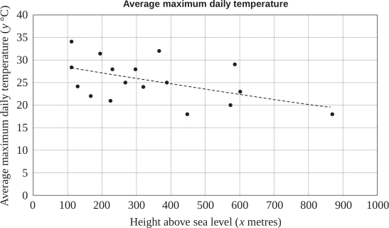
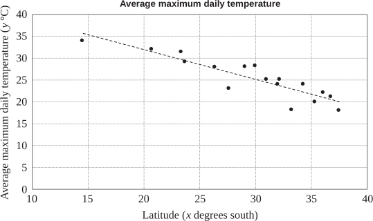
For a sample of 17 inland towns in Australia, the height above sea level, `x` (metres), and the average maximum daily temperature, `y` (°C), were recorded.

The graph shows the data as well as a regression line.


The equation of the regression line is  `y = 29.2-0.011x`.

The correlation coefficient is  `r =-0.494`.

  1. i.  By using the equation of the regression line, predict the average maximum daily temperature, in degrees Celsius, for a town that is 540 m above sea level. Give your answer correct to one decimal place.   (1 mark)

    --- 1 WORK AREA LINES (style=lined) ---
  2. ii. The gradient of the regression line is −0.011. Interpret the value of this gradient in the given context.   (2 marks)

    --- 4 WORK AREA LINES (style=lined) ---
  3. The graph below shows the relationship between the latitude, `x` (degrees south), and the average maximum daily temperature, `y` (°C), for the same 17 towns, as well as a regression line.


    The equation of the regression line is  `y = 45.6-0.683x`.
  4. The correlation coefficient is  `r =-0.897`.
  5. Another inland town in Australia is 540 m above sea level. Its latitude is 28 degrees south.
  6. Which measurement, height above sea level or latitude, would be better to use to predict this town’s average maximum daily temperature? Give a reason for your answer.   (1 mark)

    --- 2 WORK AREA LINES (style=lined) ---
Show Answers Only

a.    i.  `23.3°text(C)`

ii. `text(See Worked Solutions)`

b.    `text(Latitude. Correlation coefficient shows a stronger relationship.)`

Show Worked Solution
a.i.     `y` `=29.2-0.011(540)`
    `=23.26`
    `=23.3°text{C  (1 d.p.)`
♦♦ Mean mark (a.ii.) 28%.

 
a.ii.
`text(On average, the average maximum daily temperature of)`

`text(inland towns drops by 0.011 of a degree for every metre)`

`text(above sea level the town is situated.)`
 

♦♦♦ Mean mark (b) 18%.

b.    `text(The correlation co-efficient of the regression line using)`

`text(latitude is significantly stronger than the equivalent)`

`text(co-efficient for the regression line using height above sea)`

`text(level.)`

`:.\ text(The equation using latitude is preferred.)`

Filed Under: Bivariate Data Analysis (Y12), S4 Bivariate Data Analysis (Y12) Tagged With: 2adv-std2-common, Band 4, Band 5, Band 6, common-content, smc-6934-20-LSRL, smc-6934-30-Correlation, smc-6934-50-Gradient Interpretation, smc-785-20-Least-Squares Regression Line, smc-785-30-Correlation, smc-785-50-Gradient Interpretation

Statistics, STD2 S4 2021 HSC 28

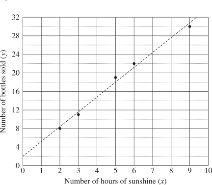
A salesperson is interested in the relationship between the number of bottles of lemonade sold per day and the number of hours of sunshine on the day.

The diagram shows the dataset used in the investigation and the least-squares regression line.


  1. Find the equation of the least-squares regression line relating to the dataset.   (2 marks)

    --- 4 WORK AREA LINES (style=lined) ---
  2. Suppose a sixth data point was collected on a day which had 10 hours of sunshine. On that day 45 bottles of lemonade were sold.
  3. What would happen to the gradient found in part (a)?   (1 mark)

    --- 2 WORK AREA LINES (style=lined) ---
Show Answers Only

a.    `y=3.2x+2`

b.    `text{Gradient would increase (steepen).}`

Show Worked Solution

a.    `text(Method 1)`

♦ Mean mark part (a) 37%.

`text{Input data points (in Stats Mode “Ax + B”):}`

`(2,8), (3, 11), (5, 19), (6, 22), (9, 30)`

`=>\ y=3.2x + 2`
 

`text(Method 2)`
 

`text{Find gradient using (0, 2) and (5, 18)}:`

`m=(18-2)/(5-0) = 3.2,\ \ ytext(-intercept)\ = 2`

`:.\ text(Equation:)\ y=3.2x + 2`

Mean mark part (b) 53%.

 
 b.    `text(Method 1)`

`text{Add (10, 45) to the data set in Stats Mode above:}`

`text(Gradient increases to 4.1.)`
 

`text(Method 2)`

`text{Data point (10, 45) lies above the regression line.`

`:.\ text{Gradient would increase (steepen).}`

Filed Under: Bivariate Data Analysis (Y12), S4 Bivariate Data Analysis (Y12) Tagged With: Band 5, common-content, smc-6934-20-LSRL, smc-6934-50-Gradient Interpretation, smc-6934-70-Calculator (Stats Mode), smc-785-20-Least-Squares Regression Line, smc-785-50-Gradient Interpretation, smc-785-70-Calculator (Stats Mode)

Statistics, STD2 S4 2020 HSC 36

A cricket is an insect. The male cricket produces a chirping sound.

A scientist wants to explore the relationship between the temperature in degrees Celsius and the number of cricket chirps heard in a 15-second time interval.

Once a day for 20 days, the scientist collects data. Based on the 20 data points, the scientist provides the information below.

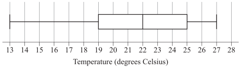
  • A box-plot of the temperature data is shown.
     
       
  • The mean temperature in the dataset is 0.525°C below the median temperature in the dataset.
  • A total of 684 chirps was counted when collecting the 20 data points.

The scientist fits a least-squares regression line using the data `(x, y)`, where  `x`  is the temperature in degrees Celsius and  `y`  is the number of chirps heard in a 15-second time interval. The equation of this line is

`y = −10.6063 + bx`,

where  `b`  is the slope of the regression line.

The least-squares regression line passes through the point  `(barx, bary)`, where  `barx`  is the sample mean of the temperature data and  `bary`  is the sample mean of the chirp data.

Calculate the number of chirps expected in a 15-second interval when the temperature is 19° Celsius. Give your answer correct to the nearest whole number.   (5 marks)

Show Answers Only

`29\ text(chirps)`

Show Worked Solution

`y =-10.6063 + bx`

♦♦♦ Mean mark 18%.

`text(Find)\ b:`

`text(Line passes through)\ \ (barx, bary)`

`barx` `= 22-0.525`
  `= 21.475`
`bary` `= text(total chirps)/text(number of data points)`
  `= 684/20`
  `= 34.2`


`34.2` `=-10.6063 + b(21.475)`
`:.b` `= 44.8063/21.475`
  `~~ 2.0864`

 
`text(If)\ \ x = 19,`

`y` `=-10.6063 + 2.0864 xx 19`
  `= 29.03`
  `= 29\ text(chirps)`

Filed Under: Bivariate Data Analysis (Y12), S4 Bivariate Data Analysis (Y12) Tagged With: 2adv-std2-common, Band 6, common-content, smc-6934-20-LSRL, smc-785-20-Least-Squares Regression Line

Statistics, STD2 S4 2020 HSC 12 MC

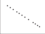
For a set of bivariate data, Pearson's correlation coefficient is  –1.

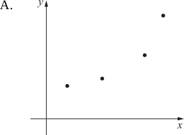
Which graph could best represent this set of bivariate data?


Show Answers Only

`D`

Show Worked Solution

`text(Negative correlation coefficient:)`

`text(Line of Best Fit will go from top left to bottom right)`

`text(Correlation coefficient of magnitude 1:)`

`text(Data will be in a straight line.)`

`=> D`

Filed Under: Bivariate Data Analysis (Y12), S4 Bivariate Data Analysis (Y12) Tagged With: Band 4, common-content, smc-6934-40-Pearson’s, smc-785-40-Pearson's

Statistics, STD2 S4 EQ-Bank 26

Ten high school students have their height and the length of their right foot measured.

The results are recorded in the table below.


  1. Using technology, calculate Pearson's correlation coefficient for the data. Give your answer to 3 decimal places.   (1 mark)

    --- 1 WORK AREA LINES (style=lined) ---
  2. Describe the strength of the association between height and length of right foot for these students.   (1 mark)

    --- 2 WORK AREA LINES (style=lined) ---
  3. Using technology, determine the least squares regression line that allows height to be predicted from right foot length.   (1 mark)

    --- 1 WORK AREA LINES (style=lined) ---
Show Answers Only

a.    `0.941\ \ (text(to 3 d.p.))`

b.    `text(The association is positive and strong.)`

c.    `text(Height) =47.4 + 4.7 xx text(foot length)`

Show Worked Solution

a.    `text(By calculator,)`

COMMENT: Issues here? YouTube has short and excellent help videos – search your calculator model and topic – eg. “fx-82 correlation” .

`r` `= 0.94095…`
  `= 0.941\ \ (text(to 3 d.p.))`

  
b.
    `text(The association is positive and strong.)`
  

c.    `x\ text(value ⇒ foot length (independent variables))`

`y\ text(value ⇒ height.)`

`text(By calculator:)`

`text(Height) = 47.4 + 4.7 xx text(foot length)`

Filed Under: Bivariate Data Analysis, Bivariate Data Analysis (Y12), S4 Bivariate Data Analysis (Y12) Tagged With: Band 4, common-content, smc-1001-20-Least-Squares Regression Line, smc-1001-30-Correlation, smc-1001-40-Pearson's, smc-1001-70-Calculator (Stats Mode), smc-6934-20-LSRL, smc-6934-30-Correlation, smc-6934-40-Pearson’s, smc-6934-70-Calculator (Stats Mode), smc-785-20-Least-Squares Regression Line, smc-785-30-Correlation, smc-785-40-Pearson's, smc-785-70-Calculator (Stats Mode)

Statistics, 2ADV S2 EQ-Bank 21

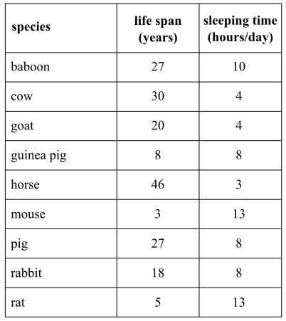
The table below lists the average life span (in years) and average sleeping time (in hours/day) of 9 animal species.


  1. Using sleeping time as the independent variable, calculate the least squares regression line.   (1 mark)

    --- 1 WORK AREA LINES (style=lined) ---
  2. A wallaby species sleeps for 4.5 hours, on average, each day.


    Use your equation from part (a) to predict its expected life span, to the nearest year.   (1 mark)

    --- 1 WORK AREA LINES (style=lined) ---
Show Answers Only

a.    `text(life span) = 42.89-2.85 xx text(sleeping time)`

b.    `30\ text(years)`

Show Worked Solution

a.    `text(By calculator:)`

COMMENT: Issues here? YouTube has short and excellent help videos – search your calculator model and topic – eg. “fx-82 regression line” .

`text(life span) = 42.89-2.85 xx text(sleeping time)`
 

b.    `text(Predicted life span of wallaby)`

`= 42.89-2.85 xx 4.5` 

`= 30.065~~ 30\ text(years)`

Filed Under: Bivariate Data Analysis, Bivariate Data Analysis (Y12), S4 Bivariate Data Analysis (Y12) Tagged With: Band 3, Band 4, common-content, smc-1001-20-Least-Squares Regression Line, smc-1001-70-Calculator (Stats Mode), smc-6934-20-LSRL, smc-6934-70-Calculator (Stats Mode), smc-785-20-Least-Squares Regression Line, smc-785-70-Calculator (Stats Mode)

Statistics, 2ADV S2 EQ-Bank 20

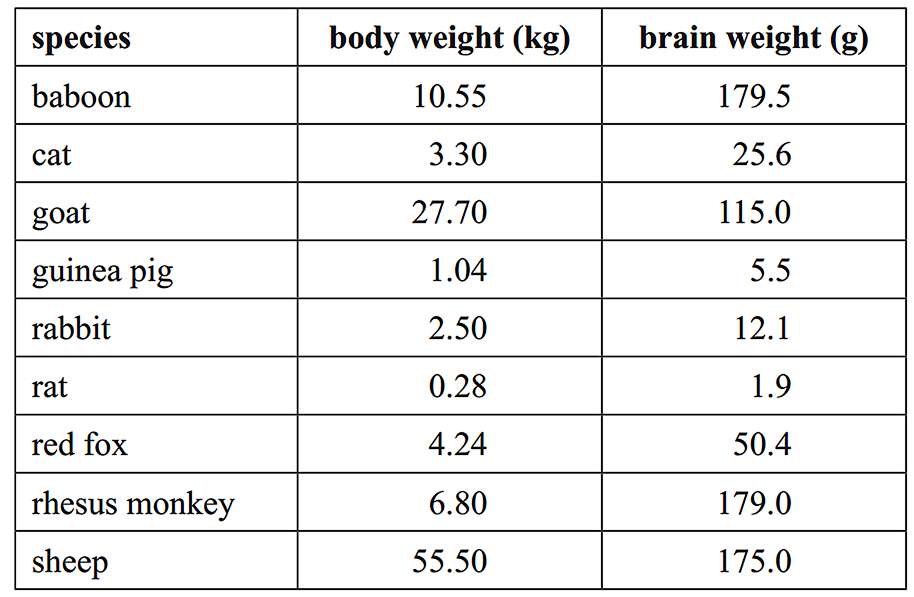
The table below lists the average body weight (in kilograms) and average brain weight (in grams) of nine animal species.


A least squares regression line is fitted to the data using body weight as the independent variable.

  1. Calculate the equation of the least squares regression line.   (1 mark)

    --- 2 WORK AREA LINES (style=lined) ---
  2. If dingos have an average body weight of 22.3 kilograms, calculate the predicted average brain weight of a dingo using your answer to part (a).   (1 mark)

    --- 1 WORK AREA LINES (style=lined) ---

Show Answers Only

a.    `text(brain weight) = 49.4 + 2.68 xx text(body weight)`

b.    `109\ text(grams)`

Show Worked Solution

a.    `text(By calculator:)`

COMMENT: Know this critical calculator skill!.

`text(brain weight) = 49.4 + 2.68 xx text(body weight)`
  

b.    `text(Predicted brain weight of a dingo)`

`= 49.4 + 2.68 xx 22.3` 

`=109.164 ~~ 109\ text(grams)`

Filed Under: Bivariate Data Analysis, Bivariate Data Analysis (Y12), S4 Bivariate Data Analysis (Y12) Tagged With: Band 3, Band 4, common-content, smc-1001-20-Least-Squares Regression Line, smc-1001-70-Calculator (Stats Mode), smc-6934-20-LSRL, smc-6934-70-Calculator (Stats Mode), smc-785-20-Least-Squares Regression Line, smc-785-70-Calculator (Stats Mode)

Statistics, 2ADV S2 EQ-Bank 22

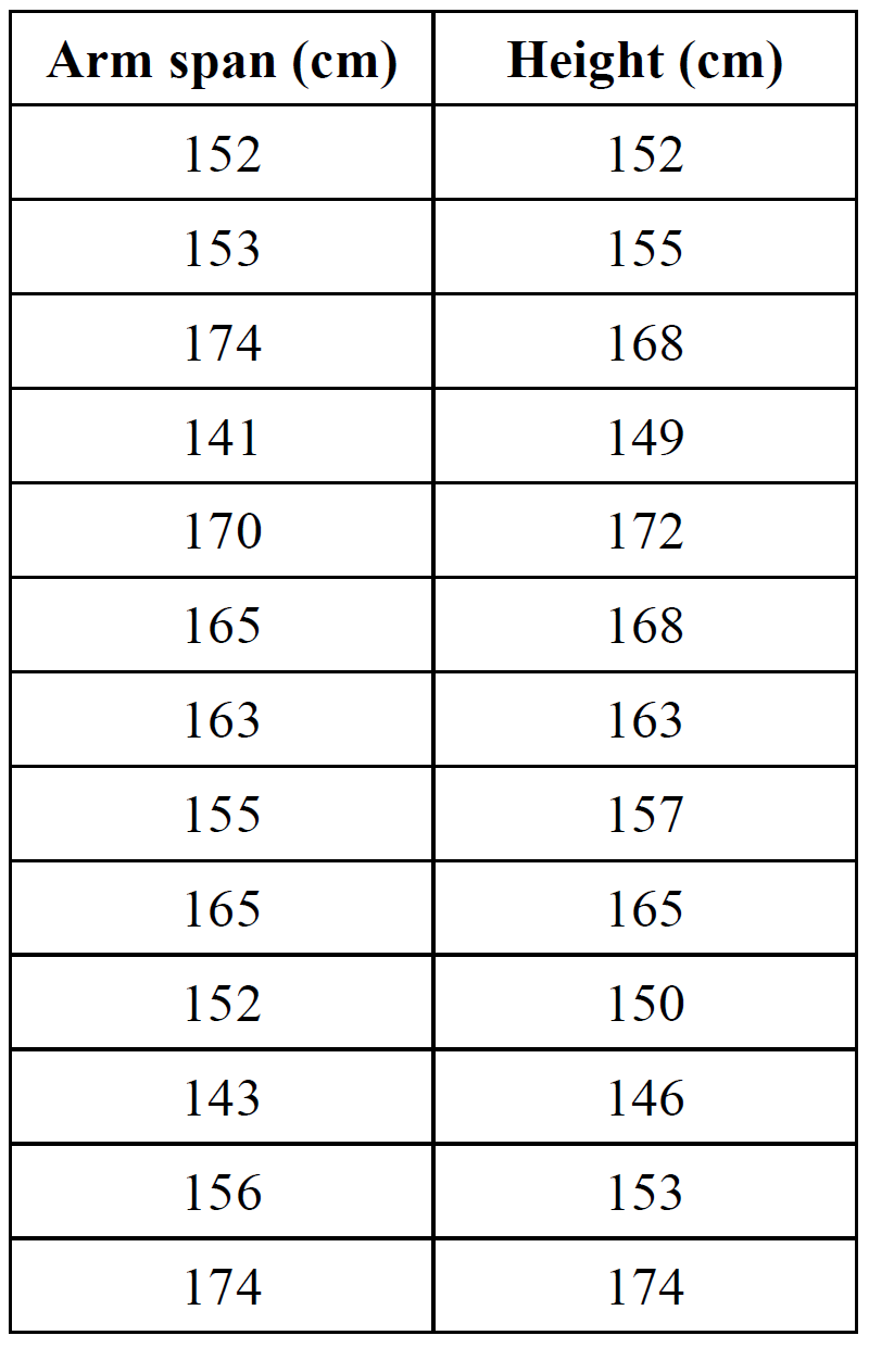
The arm spans (in cm) and heights (in cm) for a group of 13 boys have been measured. The results are displayed in the table below.
 

CORE, FUR2 2008 VCAA 4

The aim is to find a linear equation that allows arm span to be predicted from height.

  1. What will be the independent variable in the equation?   (1 mark)

    --- 1 WORK AREA LINES (style=lined) ---
  2. Assuming a linear association, determine the equation of the least squares regression line that enables arm span to be predicted from height. Write this equation in terms of the variables arm span and height. Give the coefficients correct to two decimal places.   (2 marks)

    --- 4 WORK AREA LINES (style=lined) ---
  3. Using the equation that you have determined in part b., interpret the slope of the least squares regression line in terms of the variables height and arm span.   (1 mark)

    --- 2 WORK AREA LINES (style=lined) ---
Show Answers Only

a.    `text(Height)`

b.    `text(Arm span)\ = 1.09 xx text(height)-15.63`

c.    `text(On average, arm span increases by 1.09 cm)`

`text(for each 1 cm increase in height.)`

Show Worked Solution

a.    `text(Height)`

COMMENT: Calculator skills for finding the least squares regression line were required in NESA sample exam – know this critical skill well!


b.    `text(By calculator,)`

`text(Arm span)\ = 1.09 xx text(height)-15.63`
  

c.    `text(On average, arm span increases by 1.09 cm)`

`text(for each 1 cm increase in height.)`

Filed Under: Bivariate Data Analysis, Bivariate Data Analysis (Y12), S4 Bivariate Data Analysis (Y12) Tagged With: Band 3, Band 4, common-content, smc-1001-20-Least-Squares Regression Line, smc-1001-50-Gradient Interpretation, smc-1001-70-Calculator (Stats Mode), smc-6934-20-LSRL, smc-6934-50-Gradient Interpretation, smc-6934-70-Calculator (Stats Mode), smc-785-20-Least-Squares Regression Line, smc-785-50-Gradient Interpretation, smc-785-70-Calculator (Stats Mode)

Statistics, STD2 S4 2019 HSC 23

A set of bivariate data is collected by measuring the height and arm span of seven children. The graph shows a scatterplot of these measurements.


  1. Calculate Pearson's correlation coefficient for the data, correct to two decimal places.   (1 mark)

    --- 1 WORK AREA LINES (style=lined) ---
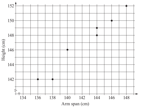
  2. Identify the direction and the strength of the linear association between height and arm span.   (1 mark)

    --- 2 WORK AREA LINES (style=lined) ---
  3. The equation of the least-squares regression line is shown.
     
               Height = 0.866 × (arm span) + 23.7
     
    A child has an arm span of 143 cm.


    Calculate the predicted height for this child using the equation of the least-squares regression line.   (1 mark)

    --- 1 WORK AREA LINES (style=lined) ---
Show Answers Only

a.    `0.98\ \ (text(2 d.p.))`

b.    `text(Direction: positive)`

`text(Strength: strong)`

c.    `147.538\ text(cm)`

Show Worked Solution

a.    `text{Use  “A + Bx”  function (fx-82 calc):}`

♦ Mean mark 40%.
COMMENT: Issues here? YouTube has short and excellent help videos – search your calculator model and topic – eg. “fx-82 correlation” .

`r` `= 0.9811…`
  `= 0.98\ \ (text(2 d.p.))`

  
b.
    `text(Direction: positive)`

`text(Strength: strong)`
  

c.     `text(Height)` `= 0.866 xx 143 + 23.7`
    `= 147.538\ text(cm)`

Filed Under: Bivariate Data Analysis, Bivariate Data Analysis (Y12), S4 Bivariate Data Analysis (Y12) Tagged With: Band 3, Band 4, Band 5, common-content, smc-1001-30-Correlation, smc-1001-40-Pearson's, smc-1001-70-Calculator (Stats Mode), smc-6934-30-Correlation, smc-6934-40-Pearson’s, smc-6934-70-Calculator (Stats Mode), smc-785-30-Correlation, smc-785-40-Pearson's, smc-785-70-Calculator (Stats Mode)

Statistics, STD2 S4 EQ-Bank 16

A student claimed that as time spent swimming training increases, the time to run a 1 kilometre time trial decreases.

After collecting and analysing some data, the student found the correlation coefficient, `r`, to be – 0.73.

What does this correlation indicate about the relationship between the time a student spends swimming training and their 1 kilometre run time trial times.   (1 mark)

--- 5 WORK AREA LINES (style=lined) ---
Show Answers Only

`text(– 0.73 indicates a strong negative relationship exists.)`

`text(In this case, it means the more time spent swimming)`

`text(training is associated with a quicker time of running a)`

`text(1 kilometre time trial.)`

Show Worked Solution

`text(– 0.73 indicates a strong negative relationship exists.)`

`text(In this case, it means the more time spent swimming)`

`text(training is associated with a quicker time of running a)`

`text(1 kilometre time trial.)`

Filed Under: Bivariate Data Analysis, Bivariate Data Analysis (Y12), S4 Bivariate Data Analysis (Y12) Tagged With: Band 3, common-content, smc-1001-30-Correlation, smc-6934-30-Correlation, smc-785-30-Correlation

Statistics, STD2 S4 2017 HSC 12 MC

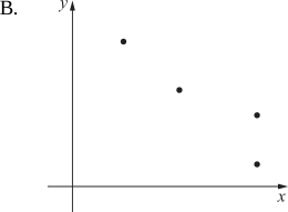
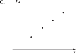
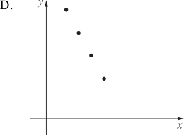
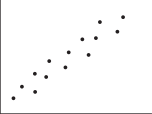
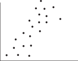
Which of the data sets graphed below has the largest positive correlation coefficient value?
 

A.      B.     
C.      D.     
Show Answers Only

\(C\)

Show Worked Solution

\(\text{Largest positive correlation occurs when both variables move}\)

\(\text{in tandem. The tighter the linear relationship, the higher the}\)

\(\text{correlation.}\)

\(\Rightarrow C\)

\(\text{(Note that B is negatively correlated)}\)

Filed Under: Bivariate Data, Bivariate Data Analysis, Bivariate Data Analysis (Y12), Correlation / Body Measurements, S3 Further Statistical Analysis (Y12), S4 Bivariate Data Analysis (Y12) Tagged With: Band 3, common-content, num-title-ct-coreb, num-title-qs-hsc, smc-1001-30-Correlation, smc-1113-30-Correlation, smc-5022-30-Correlation, smc-6934-30-Correlation, smc-785-30-Correlation

Algebra, STD2 A2 2016 HSC 29e

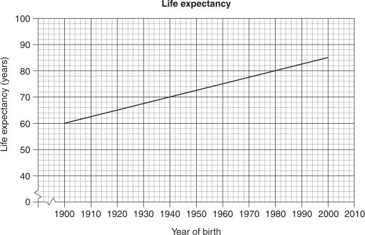
The graph shows the life expectancy of people born between 1900 and 2000.


  1. According to the graph, what is the life expectancy of a person born in 1932?   (1 mark)

    --- 1 WORK AREA LINES (style=lined) ---
  2. With reference to the value of the gradient, explain the meaning of the gradient in this context.   (2 marks)

    --- 4 WORK AREA LINES (style=lined) ---
Show Answers Only

a.    `text(68 years)`

b.    `text(After 1900, life expectancy increases 0.25 years for each later year someone is born.)`

Show Worked Solution

a.    \(\text{68 years}\)

b.    \(\text{Using (1900,60), (1980,80):}\)

\(\text{Gradient}\) \(= \dfrac{y_2-y_1}{x_2-x_1}\)
  \(= \dfrac{80-60}{1980-1900}\)
  \(= 0.25\)

 
\(\text{After 1900, life expectancy increases by 0.25 years for}\)

\(\text{each year later that someone is born.}\)

♦♦ Mean mark (b) 33%.

Filed Under: Applications of Linear Relationships, Applications of Linear Relationships, Applications: Currency, Fuel and Other Problems, Applications: Currency, Fuel and Other Problems, Bivariate Data Analysis, Bivariate Data Analysis (Y12), Life Expectancy, Other Linear Modelling, S3 Further Statistical Analysis (Y12), S4 Bivariate Data Analysis (Y12) Tagged With: Band 3, Band 5, common-content, smc-1001-10-Line of Best Fit, smc-1001-50-Gradient Interpretation, smc-1113-10-Line of Best Fit, smc-1113-50-Gradient, smc-1119-30-Other Linear Applications, smc-6256-30-Other Linear Applications, smc-6513-30-Other Linear Applications, smc-6934-10-Line of Best Fit, smc-6934-50-Gradient Interpretation, smc-785-10-Line of Best Fit, smc-785-50-Gradient Interpretation, smc-793-30-Other Linear Applications

Statistics, STD2 S4 2016 HSC 3 MC

The graph shows a scatterplot for a set of data.
 

2ug-2016-hsc-3-mc 

 
Which of the following is the best approximation for the correlation coefficient of this set of data?

  1. `−1`
  2. `−0.3`
  3. `0.3`
  4. `1`
Show Answers Only

`B`

Show Worked Solution

`text(Correlation is negative and weak.)`

`=> B`

Filed Under: Bivariate Data Analysis, Bivariate Data Analysis (Y12), Correlation / Body Measurements, S4 Bivariate Data Analysis (Y12) Tagged With: Band 4, common-content, smc-1001-30-Correlation, smc-6934-30-Correlation, smc-785-30-Correlation

Statistics, STD2 S4 2015 HSC 28e

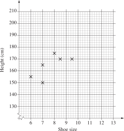
The shoe size and height of ten students were recorded.

\begin{array} {|l|c|c|}
\hline \rule{0pt}{2.5ex} \text{Shoe size} \rule[-1ex]{0pt}{0pt} & \text{6} & \text{7} & \text{7} & \text{8} & \text{8.5} & \text{9.5} & \text{10} & \text{11} & \text{12} & \text{12} \\
\hline \rule{0pt}{2.5ex} \text{Height} \rule[-1ex]{0pt}{0pt} & \text{155} & \text{150} & \text{165} & \text{175} & \text{170} & \text{170} & \text{190} & \text{185} & \text{200} & \text{195} \\
\hline
\end{array}

  1. Complete the scatter plot AND draw a line of fit by eye.   (2 marks)
     
     
  2. Use the line of fit to estimate the height difference between a student who wears a size 7.5 shoe and one who wears a size 9 shoe.   (1 mark)

    --- 1 WORK AREA LINES (style=lined) ---

  3. A student calculated the correlation coefficient to be 1 for this set of data. Explain why this cannot be correct.   (1 mark)

    --- 2 WORK AREA LINES (style=lined) ---
Show Answers Only

a.    `text(See Worked Solutions.)`

b.    `13\ text{cm  (or close given LOBF drawn)}

c.    `text(A correlation co-efficient of 1 would mean that all data points occur on the)`

`text(line of best fit which clearly isn’t the case.)`

Show Worked Solution

a.    
      2UG 2015 28e Answer

b.    `text{Shoe size 7½ gives a height estimate of 162 cm (see graph).}`

`text{Shoe size 9 gives a height estimate of 175 cm (see graph).}`

`text(Height difference)= 175-162= 13\ text{cm  (or close given LOBF)}`
 

c.    `text(A correlation co-efficient of 1 would mean that all data points)`

♦ Mean mark (c) 39%.

`text(points occur on the line of best fit which clearly isn’t the case.)`

Filed Under: Bivariate Data Analysis, Bivariate Data Analysis (Y12), Correlation / Body Measurements, S3 Further Statistical Analysis (Y12), S4 Bivariate Data Analysis (Y12) Tagged With: Band 4, Band 5, common-content, smc-1001-10-Line of Best Fit, smc-1001-30-Correlation, smc-1113-10-Line of Best Fit, smc-1113-20-Scatterplot from Table, smc-1113-30-Correlation, smc-6934-10-Line of Best Fit, smc-6934-30-Correlation, smc-785-10-Line of Best Fit, smc-785-30-Correlation

Statistics, STD2 S4 2006 HSC 27b

Each member of a group of males had his height and foot length measured and recorded. The results were graphed and a line of fit drawn.
 

  1. Why does the value of the `y`-intercept have no meaning in this situation?   (1 mark)

    --- 2 WORK AREA LINES (style=lined) ---

  2. George is 10 cm taller than his brother Harry. Use the line of fit to estimate the difference in their foot lengths.   (1 mark)

    --- 2 WORK AREA LINES (style=lined) ---
  3. Sam calculated a correlation coefficient of  −1.2  for the data. Give TWO reasons why Sam must be incorrect.   (2 marks)

    --- 5 WORK AREA LINES (style=lined) ---
Show Answers Only

a.    `text(The y-intercept occurs when)\ x = 0.\ text(It has`

`text(no meaning to have a height of 0 cm.)`

b.    `text(A 10 cm height difference means George should)`

`text(have a 3 cm longer foot.)`

c.    `text(A correlation co-efficient must be between –1 and 1.)`

`text(Foot length is positively correlated to a person’s)`

`text(height and therefore can’t be a negative value.)`

Show Worked Solution

a.    `text(The y-intercept occurs when)\ x = 0.\ text(It has)`

`text(no meaning to have a height of 0 cm.)`


b.    `text(A 20 cm height difference results in a foot length)`

`text(difference of 6 cm.)`
 

`:.\ text(A 10 cm height difference means George should)`

`text(have a 3 cm longer foot.)`


c.    `text(A correlation co-efficient must be between –1 and 1.)`

`text(Foot length is positively correlated to a person’s)`

`text(height and therefore isn’t a negative value.)`

Filed Under: Bivariate Data Analysis, Bivariate Data Analysis (Y12), Correlation / Body Measurements, S3 Further Statistical Analysis (Y12), S4 Bivariate Data Analysis (Y12) Tagged With: Band 4, Band 5, Band 6, common-content, smc-1001-10-Line of Best Fit, smc-1001-30-Correlation, smc-1113-10-Line of Best Fit, smc-1113-30-Correlation, smc-6934-10-Line of Best Fit, smc-6934-30-Correlation, smc-785-10-Line of Best Fit, smc-785-30-Correlation

Statistics, STD2 S4 2007 HSC 9 MC

Which of the following would be most likely to have a positive correlation?

  1. The population of a town and the number of schools in that town
  2. The price of petrol per litre and the number of litres of petrol sold
  3. The hours training for a marathon and the time taken to complete the marathon
  4. The number of dogs per household and the number of televisions per household
Show Answers Only

\(A\)

Show Worked Solution

\(\text{Positive correlation means that as one variable increases,}\)

\(\text{the other tends to increase also.}\)

\(\Rightarrow A\)

Filed Under: Bivariate Data, Bivariate Data Analysis, Bivariate Data Analysis (Y12), Correlation / Body Measurements, S3 Further Statistical Analysis (Y12), S4 Bivariate Data Analysis (Y12) Tagged With: Band 4, common-content, num-title-ct-coreb, num-title-qs-hsc, smc-1001-30-Correlation, smc-1113-30-Correlation, smc-5022-35-Causality, smc-6934-30-Correlation, smc-785-30-Correlation

Statistics, STD2 S4 2008 HSC 12 MC

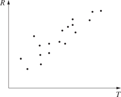
A scatterplot is shown.
 

Which of the following best describes the correlation between  \(R\)  and  \(T\)?

  1. Positive
  2. Negative 
  3. Positively skewed
  4. Negatively skewed
Show Answers Only

\(A\)

Show Worked Solution

\(\text{Correlation is positive.}\)

\(\text{NB. The skew does not directly relate to correlation.}\)

\(\Rightarrow  A\)

Filed Under: Bivariate Data, Bivariate Data Analysis, Bivariate Data Analysis (Y12), Correlation / Body Measurements, S3 Further Statistical Analysis (Y12), S4 Bivariate Data Analysis (Y12) Tagged With: Band 4, common-content, num-title-ct-coreb, num-title-qs-hsc, smc-1001-30-Correlation, smc-1113-30-Correlation, smc-5022-30-Correlation, smc-6934-30-Correlation, smc-785-30-Correlation

Statistics, STD2 S4 2014* HSC 30b

The scatterplot shows the relationship between expenditure per primary school student, as a percentage of a country’s Gross Domestic Product (GDP), and the life expectancy in years for 15 countries.


  1. For the given data, the correlation coefficient,  `r`, is 0.83. What does this indicate about the relationship between expenditure per primary school student and life expectancy for the 15 countries?   (1 mark)

    --- 1 WORK AREA LINES (style=lined) ---
  2. For the data representing expenditure per primary school student,  `Q_L`  is 8.4 and  `Q_U`  is 22.5.


    What is the interquartile range?   (1 mark)

    --- 1 WORK AREA LINES (style=lined) ---

  3. Another country has an expenditure per primary school student of 47.6% of its GDP.


    Would this country be an outlier for this set of data? Justify your answer with calculations.   (2 marks)

    --- 4 WORK AREA LINES (style=lined) ---

  4. On the scatterplot, draw the least-squares line of best fit  `y = 1.29x + 49.9`.   (2 marks)

    --- 4 WORK AREA LINES (style=lined) ---

  5. Using this line, or otherwise, estimate the life expectancy in a country which has an expenditure per primary school student of 18% of its GDP.   (1 mark)

    --- 1 WORK AREA LINES (style=lined) ---

  6. Why is this line NOT useful for predicting life expectancy in a country which has expenditure per primary school student of 60% of its GDP?   (1 mark)

    --- 1 WORK AREA LINES (style=lined) ---

Show Answers Only

a.    `text(It indicates there is a strong positive)`

`text(correlation between the two variables.)`

b.    `14.1`

c.    `text(Yes, because it’s > 43.65%)`

d.

e.    `73.1\ text(years)`

f.    `text(At 60% GDP, the line predicts a life expectancy)`

`text(of 127.3. This line of best fit is only accurate)`

`text(in a lower range of GDP expenditure.)`

Show Worked Solution

a.    `text(It indicates there is a strong positive)`

`text(correlation between the two variables)`

b.     `text(IQR)` `= Q_U\-Q_L`
    `= 22.5\-8.4= 14.1`


♦ Mean mark (c) 35% 

c.    `text(An outlier on the upper side must be more than)` 

`Q_u\ +1.5xxIQR`

`=22.5+(1.5xx14.1)`

`=\ text(43.65%)`

`:.\ text(A country with an expenditure of 47.6% is an outlier).`


d.      

e.    `text(Life expectancy) ~~ 73.1\ text{years (see dotted line)}`

♦♦ Mean mark (e) 39%

  
`text(Alternative Solution)`

`text(When)\ x=18`

`y=1.29(18)+49.9=73.12\ \ text(years)`


♦♦♦ Mean mark (f) 0%. The toughest question on the 2014 paper.
COMMENT: Examiners regularly ask students to identify and comment on outliers where linear relationships break down.

f.    `text(At 60% GDP, the line predicts a life expectancy)`

`text(of 127.3. This line of best fit is only accurate)`

`text(in a lower range of GDP expenditure.)`

Filed Under: Bivariate Data Analysis, Bivariate Data Analysis (Y12), Correlation / Body Measurements, Life Expectancy, Other Linear Modelling, S4 Bivariate Data Analysis (Y12) Tagged With: Band 4, Band 5, Band 6, common-content, smc-1001-10-Line of Best Fit, smc-1001-30-Correlation, smc-1001-60-Limitations, smc-6934-10-Line of Best Fit, smc-6934-30-Correlation, smc-6934-60-Limitations, smc-785-10-Line of Best Fit, smc-785-30-Correlation, smc-785-60-Limitations

Statistics, STD2 S4 2009 HSC 28b

The height and mass of a child are measured and recorded over its first two years. 

\begin{array} {|l|c|c|}
\hline \rule{0pt}{2.5ex} \text{Height (cm), } H \rule[-1ex]{0pt}{0pt} & \text{45} & \text{50} & \text{55} & \text{60} & \text{65} & \text{70} & \text{75} & \text{80} \\
\hline \rule{0pt}{2.5ex} \text{Mass (kg), } M \rule[-1ex]{0pt}{0pt} & \text{2.3} & \text{3.8} & \text{4.7} & \text{6.2} & \text{7.1} & \text{7.8} & \text{8.8} & \text{10.2} \\
\hline
\end{array}

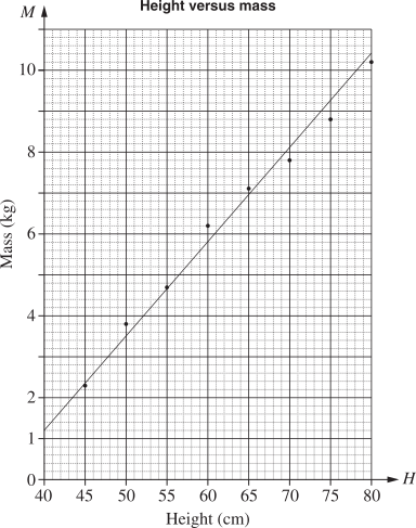
This information is displayed in a scatter graph. 
 

  1. Describe the correlation between the height and mass of this child, as shown in the graph.   (1 mark)

    --- 2 WORK AREA LINES (style=lined) ---

  2. A line of best fit has been drawn on the graph.


    Find the equation of this line.   (2 marks)

    --- 4 WORK AREA LINES (style=lined) ---

Show Answers Only

a.    `text(The correlation between height and)`

`text(mass is positive and strong.)`

b.    `M = 0.23H-8`

Show Worked Solution

a.    `text(The correlation between height and)`

♦ Mean mark (a) 48%.

`text(mass is positive and strong.)`
  

b.    `text(Using)\ \ P_1(40, 1.2)\ \ text(and)\ \ P_2(80, 10.4)`

♦♦♦ Mean mark (b) 18%. 
MARKER’S COMMENT: Many students had difficulty due to the fact the horizontal axis started at `H= text(40cm)` and not the origin.
`text(Gradient)` `= (y_2-y_1)/(x_2-x_1)`
  `= (10.4-1.2)/(80-40)`
  `= 9.2/40= 0.23`

  
`text(Line passes through)\ \ P_1(40, 1.2)`

`text(Using)\ \ \ y-y_1` `= m(x-x_1)`
`y-1.2` `= 0.23(x-40)`
`y-1.2` `= 0.23x-9.2`
`y` `= 0.23x-8`

  
`:. text(Equation of the line is)\ \ M = 0.23H-8`

Filed Under: Bivariate Data, Bivariate Data Analysis, Bivariate Data Analysis (Y12), Life Expectancy, Other Linear Modelling, S3 Further Statistical Analysis (Y12), S4 Bivariate Data Analysis (Y12) Tagged With: Band 5, Band 6, common-content, num-title-ct-coreb, num-title-qs-hsc, smc-1001-10-Line of Best Fit, smc-1001-30-Correlation, smc-1113-10-Line of Best Fit, smc-1113-30-Correlation, smc-5022-28-LOBF equations, smc-5022-30-Correlation, smc-6934-10-Line of Best Fit, smc-6934-30-Correlation, smc-785-10-Line of Best Fit, smc-785-30-Correlation

Statistics, STD2 S4 2013 HSC 28b

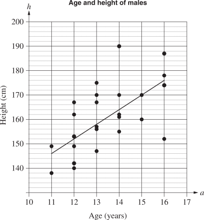
Ahmed collected data on the age (`a`) and height (`h`) of males aged 11 to 16 years.

He created a scatterplot of the data and constructed a line of best fit to model the relationship between the age and height of males.
 

  1. Determine the gradient of the line of best fit shown on the graph.   (1 mark)

    --- 2 WORK AREA LINES (style=lined) ---

  2. Explain the meaning of the gradient in the context of the data.   (1 mark)

    --- 2 WORK AREA LINES (style=lined) ---

  3. Determine the equation of the line of best fit shown on the graph.   (2 marks)

    --- 5 WORK AREA LINES (style=lined) ---

  4. Use the line of best fit to predict the height of a typical 17-year-old male.   (1 mark)

    --- 1 WORK AREA LINES (style=lined) ---

  5. Why would this model not be useful for predicting the height of a typical 45-year-old male?   (1 mark)

    --- 2 WORK AREA LINES (style=lined) ---

Show Answers Only

a.    `text(Gradient = 6)`

b.    `text(Males should grow 6 cm per year between the ages 11-16.)`

c.    `h = 6a + 80`

d.    `text(182 cm)`

e.    `text(People slow and eventually stop growing after they become adults.)`

Show Worked Solution

a.    `text{Gradient}\ =(176-146)/(16-11)=30/5=6`
 

b.    `text{Males should grow 6cm per year between the ages 11–16.}`
 

♦♦ Mean marks of 38%, 26% and 25% respectively for parts (a)-(c).

c.    `text{Gradient = 6,  Passes through (11, 146)}`

`y-y_1` `=m(x-x_1)`
`h-146` `=6(a-11)`
`h` `=6a-66+146`
  `=6a + 80`


d.   `text{Substitute}\ \ a=17\ \ \text{into equation from part (c):}`

`h=(6 xx 17) +80=182`

`:.\ text{A typical 17 year old is expected to be 182cm.}`
 

e.    `text(People slow and eventually stop growing after they become adults.)`

Filed Under: Bivariate Data Analysis, Bivariate Data Analysis (Y12), Life Expectancy, Other Linear Modelling, S3 Further Statistical Analysis (Y12), S4 Bivariate Data Analysis (Y12) Tagged With: Band 4, Band 5, common-content, smc-1001-10-Line of Best Fit, smc-1001-50-Gradient Interpretation, smc-1001-60-Limitations, smc-1113-10-Line of Best Fit, smc-1113-50-Gradient, smc-1113-60-Limitations, smc-6934-10-Line of Best Fit, smc-6934-50-Gradient Interpretation, smc-6934-60-Limitations, smc-785-10-Line of Best Fit, smc-785-50-Gradient Interpretation, smc-785-60-Limitations

Statistics, STD2 S4 2011 HSC 8 MC

In which graph would the data have a correlation coefficient closest to  – 0.9?

2UG 2011 8

Show Answers Only

`D`

Show Worked Solution

`text{Data needs to show a strong negative correlation}`

`text{(i.e. top left to lower right.)}`

`=>D`

Filed Under: Bivariate Data Analysis, Bivariate Data Analysis (Y12), Correlation / Body Measurements, S4 Bivariate Data Analysis (Y12) Tagged With: Band 4, common-content, smc-1001-30-Correlation, smc-6934-30-Correlation, smc-785-30-Correlation

Statistics, STD2 S4 2012 HSC 11 MC

Which of the following relationships would most likely show a negative correlation?

  1. The population of a town and the number of hospitals in that town. 
  2. The hours spent training for a race and the time taken to complete the race. 
  3. The price per litre of petrol and the number of people riding bicycles to work. 
  4. The number of pets per household and the number of computers per household. 
Show Answers Only

\(B\)

Show Worked Solution

\(\text{Increased hours training should reduce the time}\)

\(\text{to complete a race.}\)

\(\Rightarrow B\)

♦ Mean mark 43%.

Filed Under: Bivariate Data, Bivariate Data Analysis, Bivariate Data Analysis (Y12), Correlation / Body Measurements, S3 Further Statistical Analysis (Y12), S4 Bivariate Data Analysis (Y12) Tagged With: Band 5, common-content, num-title-ct-coreb, num-title-qs-hsc, smc-1001-30-Correlation, smc-1113-30-Correlation, smc-5022-30-Correlation, smc-5022-35-Causality, smc-6934-30-Correlation, smc-785-30-Correlation

Statistics, STD2 S4 2013 HSC 2 MC

Which graph best shows data with a correlation closest to 0.3?
 

2013 2 mc1

2013 2 mc2


Show Answers Only

`A`

Show Worked Solution

`A\ text(is correct since the data slopes bottom)`

`text{left to top right (i.e. it’s positive).}`

`D\ text(also slopes correctly but exhibits a higher)`

`text(correlation co-efficient.)`

`=>A`

Filed Under: Bivariate Data Analysis, Bivariate Data Analysis (Y12), Correlation / Body Measurements, S4 Bivariate Data Analysis (Y12) Tagged With: Band 4, common-content, smc-1001-30-Correlation, smc-6934-30-Correlation, smc-785-30-Correlation

Copyright © 2014–2026 SmarterEd.com.au · Log in