Band 4 – Page 97

CORE, FUR2 2009 VCAA 2

The time series plot below shows the rainfall (in mm) for each month during 2008.

Which month had the highest rainfall? (1 mark)

--- 1 WORK AREA LINES (style=lined) ---
Use three-median smoothing to smooth the time series. Plot the smoothed time series on the plot above.
Mark each smoothed data point with a cross (×). (2 marks)

--- 0 WORK AREA LINES (style=lined) ---
Describe the general pattern in rainfall that is revealed by the smoothed time series plot. (1 mark)

--- 3 WORK AREA LINES (style=lined) ---

Show Answers Only

`text(November)`
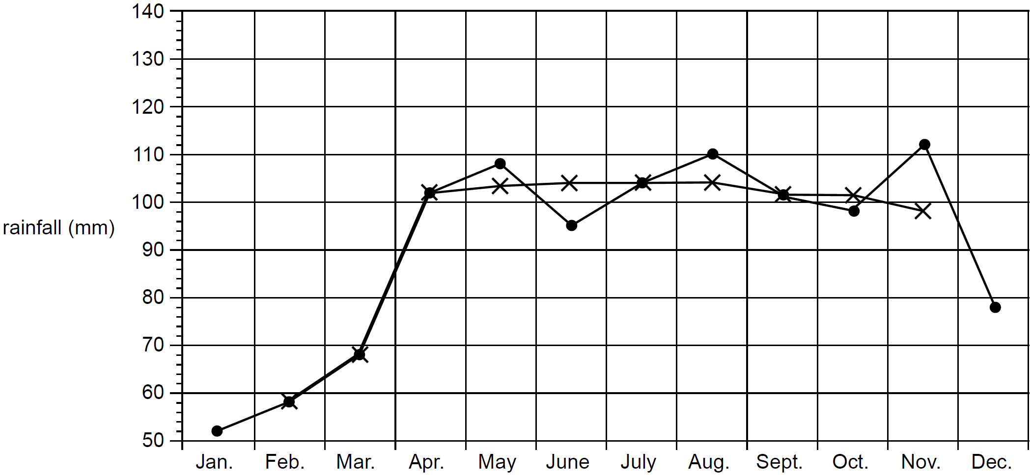
`text(Until April, the rainfall increases each month)`
`text(and then it remains relatively constant until)`
`text(November).`

Show Worked Solution

a. `text(November)`

MARKER’S COMMENT: Locate medians graphically by inspection. Explaining a general pattern with more than one trend proved challenging.

c. `text(Until April, there is an increase in rainfall)`

`text(and then it remains relatively constant until)`

`text(November.)`

MATRICES, FUR2 2015 VCAA 1

Students in a music school are classified according to three ability levels: beginner (`B`), intermediate (`I`) or advanced (`A`).

Matrix `S_0`, shown below, lists the number of students at each level in the school for a particular week.

`S_0 = [(20), (60), (40)] {:(B), (I), (A):}`

How many students in total are in the music school that week? (1 mark)

--- 1 WORK AREA LINES (style=lined) ---

The music school has four teachers, David (`D`), Edith (`E`), Flavio (`F`) and Geoff (`G`).

Each teacher will teach a proportion of the students from each level, as shown in matrix `P` below.

`{:(qquadqquadqquad{:(Dquad,Eqquad,Fqquad,G):}),(P = [(0.25,0.5,0.15,0.1)]):}`

The matrix product, `Q = S_0P`, can be used to find the number of students from each level taught by each teacher.

i. Complete matrix `Q`, shown below, by writing the missing elements in the shaded boxes. (1 mark)
--- 0 WORK AREA LINES (style=lined) ---

ii. How many intermediate students does Edith teach? (1 mark)

--- 1 WORK AREA LINES (style=lined) ---

The music school pays the teachers $15 per week for each beginner student, $25 per week for each intermediate student and $40 per week for each advanced student.

These amounts are shown in matrix `C` below.

`{:(qquad qquad quad{:(B quad, I quad,A):}),(C = [(15, 25, 40)]):}`

The amount paid to each teacher each week can be found using a matrix calculation.

i. Write down a matrix calculation in terms of `Q` and `C` that results in a matrix that lists the amount paid to each teacher each week. (1 mark)

--- 1 WORK AREA LINES (style=lined) ---
ii. How much is paid to Geoff each week? (1 mark)

--- 3 WORK AREA LINES (style=lined) ---

Show Answers Only

`120`
1. `[(5, 10, 3, 2), (15, 30, 9, 6), (10, 20, 6, 4)]`
2. `30`
1. `C xx Q`
2. `$340`

Show Worked Solution

a. `20 + 60 + 40 = 120`

b.i.	`Q`	`= S_0 P`
		`= [(20), (60), (40)] [(0.25, 0.5, 0.15, 0.1)]`
		`= [(5, 10, 3, 2), (15, 30, 9, 6), (10, 20, 6, 4)]`

b.ii. `text(Edith teaches 30 intermediate students.)`

c.i. `C xx Q`

c.ii. `CQ = [(15, 25, 40)] [(5, 10, 3, 2), (15, 30, 9, 6), (10, 20, 6, 4)]`

`:.\ text(Geoff’s pay)`

`= 15 xx 2 + 25 xx 6 + 40 xx 4`

`= $340`

CORE, FUR2 2010 VCAA 3

Table 2 shows the Australian gross domestic product (GDP) per person, in dollars, at five yearly intervals for the period 1980 to 2005.

Complete the time series plot above by plotting the GDP for the years 2000 and 2005. (1 mark)

--- 0 WORK AREA LINES (style=lined) ---
Briefly describe the general trend in the data. (1 mark)

--- 1 WORK AREA LINES (style=lined) ---

In Table 3, the variable year has been rescaled using 1980 = 0, 1985 = 5 and so on. The new variable is time.

Use the variables time and GDP to write down the equation of the least squares regression line that can be used to predict GDP from time. Take time as the independent variable. (2 marks)

--- 4 WORK AREA LINES (style=lined) ---
In the year 2007, the GDP was $34 900. Find the error in the prediction if the least squares regression line calculated in part c. is used to predict GDP in 2007. (2 marks)

--- 3 WORK AREA LINES (style=lined) ---

Show Answers Only

`text(An increasing trend.)`
`text(GDP = 20 000 + 524 × time)`
`752\ text(below the actual GDP)`

Show Worked Solution

b. `text(An increasing trend.)`

c. `text(By calculator,)`

MARKER’S COMMENT: Students are expected to use the variables in the diagram rather than just `x` and `y`.

`text(GDP) = 20\ 000 + 524 × text(time)`

d. `text(In 2007, time = 27,)`

`text{GDP (Predicted)}\ = 20\ 000 + 524 xx 27= 34\ 148`

`:.\ text(Error)\ = 34\ 900-34\ 148= 752\ \ text{(less than real GDP)}`

In the scatterplot below, average annual female income, in dollars, is plotted against average annual male income, in dollars, for 16 countries. A least squares regression line is fitted to the data.

The equation of the least squares regression line for predicting female income from male income is

female income = 13 000 + 0.35 × male income

What is the explanatory variable? (1 mark)

--- 1 WORK AREA LINES (style=lined) ---
Complete the following statement by filling in the missing information.

From the least squares regression line equation it can be concluded that, for these countries, on average, female income increases by `text($________)` for each $1000 increase in male income. (1 mark)

--- 0 WORK AREA LINES (style=lined) ---
1. Use the least squares regression line equation to predict the average annual female income (in dollars) in a country where the average annual male income is $15 000. (1 mark)
  
  --- 1 WORK AREA LINES (style=lined) ---
2. The prediction made in part c.i. is not likely to be reliable.
  
  Explain why. (1 mark)
  
  --- 2 WORK AREA LINES (style=lined) ---

Show Answers Only

`text(Male income)`
`$350`
1. `$18\ 250`
2. `text(The model established by the regression)`
  `text(equation cannot be relied upon outside the)`
  `text(range of the given data set.)`

Show Worked Solution

a. `text(Male income)`

b. `text(Increase in female income)`

`= 0.35 xx 1000`

`= $350`

c.i. `text(Average annual female income)`

`= 13\ 000 + 0.35 xx 15\ 000`

`= $18\ 250`

♦♦ This part was poorly answered (exact data unavailable).
MARKER’S COMMENT: Many students offered “real world” explanations which did not gain a mark here.

c.ii. `text(The model established by the regression)`

`text(equation cannot be relied upon outside the)`

`text(range of the given data set.)`

CORE, FUR2 2010 VCAA 1

Table 1 shows the percentage of women ministers in the parliaments of 22 countries in 2008.

What proportion of these 22 countries have a higher percentage of women ministers in their parliament than Australia? (1 mark)

--- 1 WORK AREA LINES (style=lined) ---
Determine the median, range and interquartile range of this data. (2 marks)

--- 5 WORK AREA LINES (style=lined) ---

The ordered stemplot below displays the distribution of the percentage of women ministers in parliament for 21 of these countries. The value of Canada is missing.

Complete the stemplot above by adding the value for Canada. (1 mark)

--- 1 WORK AREA LINES (style=lined) ---
Both the median and the mean appropriate measures of centre for this distribution.
Explain why. (1 mark)

--- 1 WORK AREA LINES (style=lined) ---

Show Answers Only

`0.5`
`text(Median= 28, Range = 56, IQR = 17)`
`1 | 246`
`text(S)text(ince the distribution is approximately)`

`text(symmetric, the median and mean will be)`

`text(appropriate measures of the centre.)`

Show Worked Solution

a. `11/22 = 0.5`

b. `text(22 data points,)`

`text(Median)`	`=\ text{(11th + 12th)}/2`
	`= (32 + 24)/2`
	`= 28`

`text(Range)`	`= 56 – 0`
	`= 56`

`Q_1=21 and Q_3=38`

`text(IQR)`	`= 38 – 21`
	`= 17`

c. `1 | 2 quad 4 quad 6`

♦♦ Part (d) was “poorly answered”.
MARKER’S COMMENT: The use of “symmetric” gained a mark while “evenly distributed” was deemed too vague.

d. `text(S)text(ince the distribution is approximately)`

`text(symmetric, the median and mean will be)`

`text(appropriate measures of the centre.)`

CORE, FUR2 2011 VCAA 3

The following time series plot shows the average age of women at first marriage in a particular country during the period 1915 to 1970.

Use this plot to describe, in general terms, the way in which the average age of women at first marriage in this country has changed during the period 1915 to 1970. (1 mark)

--- 3 WORK AREA LINES (style=lined) ---

During the period 1986 to 2006, the average age of men at first marriage in a particular country indicated an increasing linear trend, as shown in the time plot below.

A three-median line could be used to model this trend.

On the graph above
i. clearly mark with a cross (×) the three points that would be used to fit a three-median line to this time series plot. (2 marks)

--- 0 WORK AREA LINES (style=lined) ---
ii. draw in the three-median line. (1 mark)

--- 0 WORK AREA LINES (style=lined) ---

Show Answers Only

`text(Constant between 1915 and 1935 and then)`
`text(decreasing between 1935 and 1970.)`

Show Worked Solution

a. `text(The average age of women at first marriage was fairly)`

`text(constant between 1915 and 1935, and then decreased)`

`text(between 1935 and 1970.)`

b.i. & ii.

CORE, FUR2 2011 VCAA 2

Table 1 shows information about a particular country. It shows the percentage of women by age at first marriage, for the years 1986, 1996 and 2006.

Of the women who first married in 1986, what percentage were aged 20 to 29 years inclusive? (1 mark)

--- 2 WORK AREA LINES (style=lined) ---
Does the information in Table 1 support the opinion that, for the years 1986, 1996 and 2006, the age of women at first marriage was associated with years of marriage?
Justify your answer by quoting appropriate percentages. It is sufficient to consider one age group only when justifying your answer. (2 marks)
--- 4 WORK AREA LINES (style=lined) ---

Show Answers Only

`text(65.5%)`
`text(Yes. See Worked solutions.)`

Show Worked Solution

a. `text(Percentage aged 20 – 29 who married in 1986)`

`=42.1 + 23.4`

`= 65.5 text(%)`

b. `text(Yes.)`

`text(Considering the 25 – 29 age group, the)`

`text{percentage of women increased from 23.4%}`

`text{(1986), to 31.7% (1996), to 34.5% (2006).}`

CORE, FUR2 2011 VCAA 1

The stemplot in Figure 1 shows the distribution of the average age, in years, at which women first marry in 17 countries.

For these countries, determine
1. the lowest average age of women at first marriage (1 mark)
  
  --- 1 WORK AREA LINES (style=lined) ---
2. the median average age of women at first marriage (1 mark)
  
  --- 1 WORK AREA LINES (style=lined) ---

The stemplot in Figure 2 shows the distribution of the average age, in years, at which men first marry in 17 countries.

For these countries, determine the interquartile range (IQR) for the average age of men at first marriage. (1 mark)

--- 3 WORK AREA LINES (style=lined) ---
If the data values displayed in Figure 2 were used to construct a boxplot with outliers, then the country for which the average age of men at first marriage is 26.0 years would be shown as an outlier.
Explain why is this so. Show an appropriate calculation to support your explanation. (2 marks)

--- 4 WORK AREA LINES (style=lined) ---

Show Answers Only

1. `text(25 years)`
2. `text(28.2 years)`
`text(1.1 years)`
`text(See Worked Solutions)`

Show Worked Solution

a.i. `text(Lowest age = 25 years)`

a.ii. `text(Median age of 17 data point is the)`

`text(9th point = 28.2 years)`

b. `Q_L = 29.9, Q_U = 31.0,`

`:. IQR`	`= Q_U − Q_L`
	`= 31.0 − 29.9`
	`= 1.1\ text(years)`

c. `1.5 xx IQR = 1.5 xx 1.1 = 1.65`

MARKER’S COMMENT: Many students correctly calculated 28.25 but then failed to discuss how 26.0 related to it.

`Q_1 – IQR`	`=29.9-1.65`
	`=28.25`

`text(S)text(ince 26.0 < 28.25,)`

`:. 26.0\ text(is an outlier.)`

CORE, FUR2 2012 VCAA 4

The wind speeds (in km/h) that were recorded at the weather station at 9.00 am and 3.00 pm respectively on 18 days in November are given in the table below. A scatterplot has been constructed from this data set.

Let the wind speed at 9.00 am be represented by the variable ws9.00am and the wind speed at 3.00 pm be represented by the variable ws3.00pm.

The relationship between ws9.00am and ws3.00pm shown in the scatterplot above is nonlinear.

A squared transformation can be applied to the variable ws3.00pm to linearise the data in the scatterplot.

Apply the squared transformation to the variable ws3.00pm and determine the equation of the least squares regression line that allows (ws3.00pm)² to be predicted from ws9.00am.

In the boxes provided, write the coefficients for this equation, correct to one decimal place. (2 marks)

--- 0 WORK AREA LINES (style=lined) ---
Use this equation to predict the wind speed at 3.00 pm on a day when the wind speed at 9.00 am is 24 km/h.

Write your answer, correct to the nearest whole number. (1 mark)

--- 3 WORK AREA LINES (style=lined) ---

Show Answers Only

`(ws3.00p m)^2 = 3.4 + 6.6 xx ws9.00am`
`13`

Show Worked Solution

a. `text(By Calculator,)`

MARKER’S COMMENT: Many students were unable to deal with the squared transformation.

`(ws3.00p m)^2 = 3.4 + 6.6 xx ws9.00am`

b. `text(Substitute)\ \ ws9.00am = 24\ \ text(into the equation:)`

`(ws3.00p m)^2=3.4+6.6 xx 24=161.8`

`:. ws3.00p m≈ 12.720… =13\ \ text{(nearest whole)}`

CORE, FUR2 2012 VCAA 3

A weather station records the wind speed and the wind direction each day at 9.00 am.

The wind speed is recorded, correct to the nearest whole number.

The parallel boxplots below have been constructed from data that was collected on the 214 days from June to December in 2011.

Complete the following statements.
The wind direction with the lowest recorded wind speed was ________.
The wind direction with the largest range of recorded wind speeds was _______. (1 mark)

--- 0 WORK AREA LINES (style=lined) ---
The wind blew from the south on eight days.
Reading from the parallel boxplots above we know that, for these eight wind speeds, the

first quartile	`Q_1 = 2\ text(km/h)`
median	`M = 3.5\ text(km/h)`
third quartile	`Q_3 = 4\ text(km/h)`

Given that the eight wind speeds were recorded to the nearest whole number, write down the eight wind speeds. (1 mark)
--- 4 WORK AREA LINES (style=lined) ---

Show Answers Only

`text(South-East and North East.)`
`2, 2, 2, 3, 4, 4, 4, 4`

Show Worked Solution

a. `text(South-East and North-East.)`

b. `text(S)text(ince the boxplot has no whiskers and the median is 3.5,)`

`text(the data set is {2, _ , _ , 3, 4, _ , _ , 4})`

♦♦ MARKER’S COMMENT: Although specific data isn’t available, “few” students answered this part correctly.

`text(S)text(ince)\ Q_1=2\ text(and is the mid-point of the 2nd and)`

`text(3rd points, both must be 2.)`

`text(Similarly,)\ Q_3=4,\ text(so the 6th and 7th points are both 4.)`

`:.\ text(The data set is:)\ {2, 2, 2, 3, 4, 4, 4, 4}`

CORE, FUR2 2012 VCAA 2

The maximum temperature and the minimum temperature at this weather station on each of the 30 days in November 2011 are displayed in the scatterplot below.

The correlation coefficient for this data set is `r = 0.630`.

The equation of the least squares regression line for this data set is

maximum temperature = `13 + 0.67` × minimum temperature

Draw this least squares regression line on the scatterplot above. (1 mark)

--- 0 WORK AREA LINES (style=lined) ---
Interpret the vertical intercept of the least squares regression line in terms of maximum temperature and minimum temperature. (1 mark)

--- 2 WORK AREA LINES (style=lined) ---
Describe the relationship between the maximum temperature and the minimum temperature in terms of strength and direction. (1 mark)

--- 2 WORK AREA LINES (style=lined) ---
Interpret the slope of the least squares regression line in terms of maximum temperature and minimum temperature. (1 mark)

--- 2 WORK AREA LINES (style=lined) ---
Determine the percentage of variation in the maximum temperature that may be explained by the variation in the minimum temperature.
Write your answer, correct to the nearest percentage. (1 mark)

--- 2 WORK AREA LINES (style=lined) ---

On the day that the minimum temperature was 11.1 °C, the actual maximum temperature was 12.2 °C.

Determine the residual value for this day if the least squares regression line is used to predict the maximum temperature.
Write your answer, correct to the nearest degree. (2 marks)

--- 4 WORK AREA LINES (style=lined) ---

Show Answers Only

`text(See Worked Solutions)`
`text(On average, when the minimum temperature is)`
`text(0 °C, the maximum temperature is 13 °C)`
`text(Moderate and positive.)`
`text(On average, it is predicted that the maximum)`
`text(temperature increases by 0.67 °C for every 1 °C)`
`text(increase in the minimum temperature.)`
`40text(%)`
`-8^@text(C)`

Show Worked Solution

a. `text(The two widest points in this data range are,)`

`text{(0, 13) and (20, 26.4).}`

b. `text(On average, when the minimum temperature is)`

`text(0 °C, the maximum temperature is 13 °C.)`

♦ Parts (i) to (vi) have an average mean mark of 41%.

c. `text(Given)\ r = 0.630,`

`text(Strength: moderate)`

`text(Direction: positive)`

d. `text(On average, it is predicted that \the maximum)`

`text(temperature increases by 0.67 °C for every 1 °C)`

`text(increase in the minimum temperature.)`

e.	`r^2`	`= 0.630^2`
		`=0.3969`
		`=40text{% (nearest %)}`

f. `text(When the minimum temperature was)\ 11.1 text(°C),`

MARKER’S COMMENT: Students had particular difficulty with this part, with many using the incorrect calculation of 12.2 – 11.1 = 1.1.

`text(Predicted Value)`	`= 13 + 0.67 xx 11.1`
	`=20.437…`

`:.\ text(Residual)`	`= 12.2 − 20.437…`
	`= – 8.237…`
	`= – 8\ text{°C (nearest degree)}`

CORE, FUR2 2012 VCAA 1

The dot plot below displays the maximum daily temperature (in °C) recorded at a weather station on each of the 30 days in November 2011.

From this dot plot, determine
i. the median maximum daily temperature, correct to the nearest degree (1 mark)

--- 2 WORK AREA LINES (style=lined) ---
ii. the percentage of days on which the maximum temperature was less than 16 °C.
Write your answer, correct to one decimal place. (1 mark)

--- 3 WORK AREA LINES (style=lined) ---

Records show that the minimum daily temperature for November at this weather station is approximately normally distributed with a mean of 9.5 °C and a standard deviation of 2.25 °C.

Determine the percentage of days in November that are expected to have a minimum daily temperature less than 14 °C at this weather station.
Write your answer, correct to one decimal place. (1 mark)

--- 4 WORK AREA LINES (style=lined) ---

Show Answers Only

1. `20 text(°C)`
2. `23.3text(%)`
`97.5text(%)`

Show Worked Solution

a.i. `text(The median is the average of the 15th and 16th)`

`\ \ text{data points (30 data points in total).}`.

`:.\ text(Median = 20 °C)`

a.ii. `text{Percentage of days less than 16 °C}`

`= 7/30 xx 100text(%)`

`=23.333…`

`=23.3text{% (to 1 d.p.)}`

b.	`z text{-score (14)}`	`=(x-barx)/s`
		`=(14-9.5)/2.25`
		`=2`

`text(Percentage of days with a minimum below 14 °C)`

`= 95text(%) + 2.5text(%)`

`= 97.5text(%)`

CORE, FUR2 2013 VCAA 4

The time series plot below shows the average pay rate, in dollars per hour, for workers in a particular country for the years 1991 to 2005.

A three median line will be used to model the increasing trend in the average pay rate shown in this time series.

The explanatory variable to be used is year.

Three medians will be used to draw the three median line.
1. On the time series plot above, mark the location of each of the three medians with a cross (`X`). (2 marks)
2. Draw the three median line on the time series plot. (1 mark)
Calculate the slope of the three median line.

Write your answer, correct to one decimal place. (1 mark)
Interpret the slope of the three median line in terms of the relationship between the variables average pay rate and year. (1 mark)

Show Answers Only

i. & ii. `text(See Worked Solutions)`
`0.8`
`text(The average pay rate increases, on average,)`

`text(by $0.80 each year between 1991 and 2005.)`

Show Worked Solution

a.i. & ii. `text(The three medians points are)`

♦ Mean mark 45%.
MARKER’S COMMENT: Few students found the correct middle point.

`(1993,13.7), (1998,16.7), (2003,21.8)`

♦♦ Parts (ii) and (iii) produced an overall mean mark of 32%.

b.	`text(Slope)`	`=(y_2-y_1)/(x_2-x_1)`
		`=(21.8 − 13.7)/(2003 − 1993)`
		`= 0.81`
		`=0.8\ \ text{(to 1 d.p.)}`

MARKER’S COMMENT: Answering “an increase of 0.8 each year” received no marks (refer to actul units).

c. `text(The average pay rate increases, on average,)`

`text(by $0.80 each year between 1991 and 2005.)`

CORE, FUR2 2013 VCAA 3

The development index and the average pay rate for workers, in dollars per hour, for a selection of 25 countries are displayed in the scatterplot below.

The table below contains the values of some statistics that have been calculated for this data.

Determine the standardised value of the development index (`z` score) for a country with a development index of 91.
Write your answer, correct to one decimal place. (1 mark)

--- 3 WORK AREA LINES (style=lined) ---
Use the information in the table to show that the equation of the least squares regression line for a country’s development index, `y`, in terms of its average pay rate, `x`, is given by
`y = 81.3 + 0.272x` (2 marks)

--- 4 WORK AREA LINES (style=lined) ---
The country with an average pay rate of $14.30 per hour has a development index of 83.
Determine the residual value when the least squares regression line given in part (b) is used to predict this country’s development index.
Write your answer, correct to one decimal place. (2 marks)

--- 4 WORK AREA LINES (style=lined) ---

Show Answers Only

`1.8`
`text(See Worked Solutions)`
`−2.2`

Show Worked Solution

MARKER’S COMMENT: Many students made a careless error by using the Average pay rate (`x`-variable).

a.	`z`	`= (y-bar y)/s`
		`= (91-85.6)/2.99`
		`=1.806…`
		`= 1.8\ \ text{(to 1 d.p.)}`

♦ Parts (b) and (c) had a combined mean mark of 48%.

b.	`b`	`= r xx s_y/s_x`
		`= 0.488 xx 2.99/5.37`
		`=0.2717…`

`a`	`= bary-b barx`
	`= 85.6-0.272 xx 15.7`
	`= 81.329…`

`:.\ text(The least squares line is)`

`y = 81.3 + 0.272x`

c.	`text(Predicted)`	`= 81.3 + 0.272 xx 14.30`
		`= 85.1896…`

`:.\ text(Residual)`	`= 83-85.1896…`
	`=-2.1896…`
	`= – 2.2`

CORE, FUR2 2013 VCAA 2

The development index for each country is a whole number between 0 and 100.

The dot plot below displays the values of the development index for each of the 28 countries that has a high development index.

Using the information in the dot plot, determine each of the following. (1 mark)

--- 0 WORK AREA LINES (style=lined) ---
Write down an appropriate calculation and use it to explain why the country with a development index of 70 is an outlier for this group of countries. (2 marks)

--- 5 WORK AREA LINES (style=lined) ---

Show Answers Only

`text(Mode = 78, Range = 9)`
`text(See Worked Solutions)`

Show Worked Solution

a. `text(Mode = 78)`

`text(Range = 79 − 70 = 9)`

b. `text(An outlier occurs if a data point is below)`

`Q_1 − 1.5 xx IQR`

`Q_1 = 75, \ \ Q_3 = 78, and IQR = 78-75=3`

`:. Q_1 − 1.5 xx IQR`	`= 75 − 1.5 xx 3`
	`= 70.5`

`:. 70\ text{is an outlier (70 < 70.5)}`

CORE, FUR2 2014 VCAA 4

The scatterplot below shows the population density, in people per square kilometre, and the area, in square kilometres, of 38 inner suburbs of the same city.

For this scatterplot, `r^2 = 0.141`

Describe the association between the variables population density and area for these suburbs in terms of strength, direction and form. (1 mark)

--- 3 WORK AREA LINES (style=lined) ---
The mean and standard deviation of the variables population density and area for these 38 inner suburbs are shown in the table below.
i. One of these suburbs has a population density of 3082 people per square kilometre.
Determine the standard `z`-score of this suburb’s population density.
Write your answer, correct to one decimal place. (1 mark)

--- 3 WORK AREA LINES (style=lined) ---

Assume the areas of these inner suburbs are approximately normally distributed.

ii. How many of these 38 suburbs are expected to have an area that is two standard deviations or more above the mean?
Write your answer, correct to the nearest whole number. (1 mark)

--- 1 WORK AREA LINES (style=lined) ---
iii. How many of these 38 inner suburbs actually have an area that is two standard deviations or more above the mean? (1 mark)

--- 3 WORK AREA LINES (style=lined) ---

Show Answers Only

`text(The association is weak, negative and linear.)`
1. `− 0.8`
2. `1`
3. `2`

Show Worked Solution

♦♦ Mean mark 30%.
MARKER’S COMMENT: The most common error was to describe the association as positive.

a.	`r`	`= −sqrt(0.141)`
		`= −0.3755`

`:.\ text(The association is weak, negative and linear.)`

b.i	`z`	`=(x-bar x)/s`
		`= (3082-4370)/1560`
		`= -0.82…`
		`= -0.8\ \ text{(to 1 d.p.)}`

b.ii. `2.5text(%) xx 38 =0.95=1\ text{(nearest whole)}`

b.iii. `text{Area size (2 std deviation above mean)}`

♦♦ Very few students answered this part correctly.

`= 3.4 + 2 xx 1.6`

`=6.6\ text(km²)`

`:.\ text{From the graph, 2 inner suburbs have an area}`

`text(2 standard deviations above the mean.)`

CORE, FUR2 2014 VCAA 2

The scatterplot below shows the population and area (in square kilometres) of a sample of inner suburbs of a large city.

The equation of the least squares regression line for the data in the scatterplot is

population = 5330 + 2680 × area

Write down the response variable. (1 mark)

--- 1 WORK AREA LINES (style=lined) ---
Draw the least squares regression line on the scatterplot above. (1 mark)

--- 0 WORK AREA LINES (style=lined) ---
Interpret the slope of this least squares regression line in terms of the variables area and population. (2 marks)

--- 4 WORK AREA LINES (style=lined) ---
Wiston is an inner suburb. It has an area of 4 km² and a population of 6690.
The correlation coefficient, `r`, is equal to 0.668
i. Calculate the residual when the least squares regression line is used to predict the population of Wiston from its area. (1 mark)

--- 2 WORK AREA LINES (style=lined) ---
ii. What percentage of the variation in the population of the suburbs is explained by the variaton in area.
Write your answer, correct to one decimal place. (1 mark)

--- 2 WORK AREA LINES (style=lined) ---

Show Answers Only

`text(Population.)`
`text(Population increases by 2680 people, on average,)`
`text(for each additional 1 km² in area.)`
1. ` −9360`
2. `text(44.6%)`

Show Worked Solution

a. `text(Population.)`

♦ Mean mark 36%.
MARKER’S COMMENT: Use the equation to draw the line and use points at the extremities.

c. `text(Population increases by 2680 people, on average,)`

♦ Mean mark 41% (part (iii)).

`text(for each additional 1 km² in area.)`

d.i. `text(Predicted population) = 5330 + 2680 xx 4= 16\ 050`

`:.\ text(Residual)\ = 6690-16\ 050= -9360`

♦ Part (iv) in total had a mean mark 42%.

d.ii.	`r`	`= 0.668^2`
	`r^2`	`= 0.4462…`
		`= 44.6 text{% (to 1 d.p.)}`

`:.\ text(44.6% of the variation in the population is explained)`

`text(by variation in the area.)`

CORE, FUR2 2014 VCAA 1

The segmented bar chart below shows the age distribution of people in three countries, Australia, India and Japan, for the year 2010.

Write down the percentage of people in Australia who were aged 0 – 14 years in 2010.
Write your answer, correct to the nearest percentage. (1 mark)

--- 1 WORK AREA LINES (style=lined) ---
In 2010, the population of Japan was 128 000 000.
How many people in Japan were aged 65 years and over in 2010? (1 mark)

--- 3 WORK AREA LINES (style=lined) ---
From the graph above, it appears that there is no association between the percentage of people in the 15 – 64 age group and the country in which they live.
Explain why, quoting appropriate percentages to support your explanation. (1 mark)

--- 4 WORK AREA LINES (style=lined) ---

Show Answers Only

`text(19%)`
`29\ 440\ 000`
`text(The percentages of people in the 15 – 64 age group)`
`text(in each country is: Australia 67%, India 64%, and)`
`text(Japan 64%.)`
`text(S)text(ince the percentages are very close no matter which)`
`text(country this age group belonged to, there is no association.)`

Show Worked Solution

a. `text(19%)`

b. `text(From the graph, 23% of Japan’s population is 65 or over.)`

`:.\ text(The number of people 65 or over)`

`=128\ 000\ 000 xx 23/100`

`= 29\ 440\ 000`

c. `text(The percentages of people in the 15 – 64 age group)`

♦ Mean mark 41%.

`text(in each country is: Australia 67%, India 64%, and)`

`text(Japan 64%.)`

`text(S)text(ince the percentages are very close no matter which)`

`text(country this age group belonged to, there is no association.)`

CORE, FUR2 2015 VCAA 5

The time series plot below displays the life expectancy, in years, of people living in Australia and the United Kingdom (UK) for each year from 1920 to 2010.

By how much did life expectancy in Australia increase during the period 1920 to 2010?
Write your answer correct to the nearest year. (1 mark)

--- 2 WORK AREA LINES (style=lined) ---
In 1975, the life expectancies in Australia and the UK were very similar.
From 1975, the gap between the life expectancies in the two countries increased, with people in Australia having a longer life expectancy than people in the UK.
To investigate the difference in life expectancies, least squares regression lines were fitted to the data for both Australia and the UK for the period 1975 to 2010.
The results are shown below.

The equations of the least squares regression lines are as follows.

`text(Australia:)\ \ \ `	`text(life expectancy) = – 451.7 + 0.2657 xx text(year)`
`text(UK:)`	`text(life expectancy) = – 350.4 + 0.2143 xx text(year)`

Use these equations to predict the difference between the life expectancies of Australia and the UK in 2030.
Give your answer correct to the nearest year. (2 marks)

--- 4 WORK AREA LINES (style=lined) ---
Explain why this prediction may be of limited reliability. (1 mark)

--- 3 WORK AREA LINES (style=lined) ---

Show Answers Only

`text(22 years)`
1. `3\ text(years)`
2. `text(The year 2030 is outside the available range)`
  
  `text(of data and therefore its predictions may)`
  
  `text(become unreliable.)`

Show Worked Solution

a. `text{The increase in life expectancy (1920 – 2010)}`

`=82-60`

`=22\ text(years)`

b.i.	`text{Life expectancy (Aust)}`	`= −451.7 + 0.2657× 2030`
		`= 87.67…\ text(years)`

	`text{Life expectancy (UK)}`	`= −350.4 + 0.2143× 2030`
		`=84.62…\ text(years)`

`:.\ text(Difference)`	`= 87.67…-84.62…`
	`= 3\ text(years)\ \ \ text{(nearest year)}`

♦ Mean mark 45%.
MARKER’S COMMENT: Relate answers directly to the limitations of the given statistical data rather than future events in (b)(ii).

b.ii. `text(The year 2030 is outside the available range)`

`\ text(of data and therefore its predictions may)`

`\ text(become unreliable.)`

CORE, FUR2 2015 VCAA 4

The table below shows male life expectancy (male) and female life expectancy (female) for a number of countries in 2013. The scatterplot has been constructed from this data.

Use the scatterplot to describe the association between male life expectancy and female life expectancy in terms of strength, direction and form. (1 mark)

--- 3 WORK AREA LINES (style=lined) ---
Determine the equation of a least squares regression line that can be used to predict male life expectancy from female life expectancy for the year 2013.

Complete the equation for the least squares regression line below by writing the intercept and slope in the space provided.

Write these values correct to two decimal places. (1 mark)

--- 0 WORK AREA LINES (style=lined) ---

male = ______________ + ______________ × female

Show Answers Only

`text(Strong, positive and linear.)`
`text(male) = 9.69 + 0.81 xx text(female)`

Show Worked Solution

a. `text(Strong, positive and linear.)`

♦ Mean mark 49%.
MARKER’S COMMENT: Common errors included using the 1st column as the independent (`x`) variable and poor rounding.

b. `text(By calculator,)`

`text(male) = 9.69 + 0.81 xx text(female)`

Probability, 2UG SM-Bank 01 MC

A circle has 5 equally spaced points on its circumference, as shown.

How many different triangles using 3 of these points as vertices can be drawn? (3 marks)

A. `60`

B. `20`

C. `15`

D. `10`

Show Answers Only

`D`

Show Worked Solution

`text(Number of possible triangles)`

STRATEGY: The number of triangles is divided by `(3 xx 2 xx 1)` because the selections of any 3 vertices are unordered.

`= (5 xx 4 xx 3)/(3 xx 2 xx1)`

`= 10`

`=> D`

Financial Maths, 2ADV M1 SM-Bank 10 MC

The graph above shows the first six terms of a sequence.

This sequence could be

an arithmetic sequence that sums to one.
an arithmetic sequence with a common difference of one.
a geometric sequence with an infinite sum of one.
a geometric sequence with a common ratio of one.

Show Answers Only

`D`

Show Worked Solution

`text(Series is 1, 1, 1, …)`

`text(The only possibility within the choices)`

`text(is a geometric sequence where)\ \ r=1.`

`=> D`

CORE, FUR2 2015 VCAA 3

The scatterplot below plots male life expectancy (male) against female life expectancy (female) in 1950 for a number of countries. A least squares regression line has been fitted to the scatterplot as shown.

The slope of this least squares regression line is 0.88

Interpret the slope in terms of the variables male life expectancy and female life expectancy. (1 mark)

--- 3 WORK AREA LINES (style=lined) ---

The equation of this least squares regression line is

male = 3.6 + 0.88 × female

In a particular country in 1950, female life expectancy was 35 years.

Use the equation to predict male life expectancy for that country. (1 mark)

--- 2 WORK AREA LINES (style=lined) ---
The coefficient of determination is 0.95

Interpret the coefficient of determination in terms of male life expectancy and female life expectancy. (1 mark)

--- 4 WORK AREA LINES (style=lined) ---

Show Answers Only

`text(A slope of 0.88 means that for each year that a)`
`text(female lives longer in a particular country, a male)`
`text(in that country, on average, will tend to live 0.88)`
`text(of a year longer.)`
`34.4\ text(years)`
`text(This figure means that 95% of the variability in)`
`text(the male life expectancy can be explained by the)`
`text(variation in female life expectancy.)`

Show Worked Solution

a. `text(A slope of 0.88 means that for each year)`

♦ Mean mark 40%.
MARKER’S COMMENT: Many students did not describe the slope, despite being specifically asked about it!

`text(that a female lives longer in a particular)`

`text(country, a male in that country, on average,)`

`text(will tend to live 0.88 of a year longer.)`

b. `text(Male life expectancy)`

`=3.6 + 0.88 xx 35`

`=34.4\ text(years)`

c. `text(This figure means that 95% of the variability)`

MARKER’S COMMENT: A common error: use of `r^2 = 90.25 text(%)` as the basis of the interpretation.

`text(in the male life expectancy can be explained)`

`text(by the variation in female life expectancy.)`

CORE, FUR2 2015 VCAA 1

The histogram below shows the distribution of life expectancy of people for 183 countries.

For this distribution, the modal interval is ___________ (1 mark)

--- 0 WORK AREA LINES (style=lined) ---
In how many of these countries is life expectancy less than 55 years? (1 mark)

--- 2 WORK AREA LINES (style=lined) ---
In what percentage of these 183 countries is life expectancy between 75 and 80 years?
Write your answer correct to one decimal place. (1 mark)

--- 3 WORK AREA LINES (style=lined) ---

Show Answers Only

`text(70 – 75)`
`14`
`text(16.4%)`

Show Worked Solution

a. `text(70 – 75)`

MARKER’S COMMENT: 40% of students answered this basic question incorrectly.

b. `text(Adding up the first 2 columns,)`

`5 + 9 = 14\ text(countries)`

c. `text(% Countries with life expectancy between 75-80)`

MARKER’S COMMENT: Answers of 16% or an unrounded figure received no marks.

`= text(Number of 75-80 countries)/text(Total countries)`

`=30/183 xx 100text(%)`

`=16.39…`

`=16.4text{% (to 1 d.p.)}`

NETWORKS, FUR1 2015 VCAA 4 MC

The arrows on the diagram below show the direction of the flow of waste through a series of pipelines from a factory to a waste dump.

The numbers along the edges show the number of megalitres of waste per week that can flow through each section of pipeline.

The minimum cut is shown as a dotted line.

The capacity of this cut, in megalitres of waste per week, is

A. `6`

B. `18`

C. `26`

D. `32`

E. `34`

Show Answers Only

`C`

Show Worked Solution

`text{Minimum Cut (ML/week)}`

`= 5 + 2 + 12 + 7`

`= 26`

`=> C`

MATRICES, FUR1 2015 VCAA 6 MC

A carpenter can make four coffee tables and seven stools in a total of 33 hours.

The carpenter can make two coffee tables and three pencil boxes in a total of 12 hours.

The carpenter can make five stools and one pencil box in a total of 10 hours.

The time, in hours, that it takes to make one coffee table is closest to

A. 2

B. 3

C. 4

D. 5

E. 6

Show Answers Only

`D`

Show Worked Solution

`[(4,7,0),(2,0,3),(0,5,1)][(C),(S),(P)] = [(33),(12),(10)]`

`[(C),(S),(P)]`	`= [(4,7,0),(2,0,3),(0,5,1)]^(−1)[(33),(12),(10)]`
	`= [(4.99),(1.86),(0.68)]`

`:.\ text(One coffee table takes 5 hours)`

`=> D`

MATRICES, FUR1 2015 VCAA 5 MC

Wendy buys one type of flower each day.

She chooses from tulips (`T`), roses (`R`), carnations (`C`), irises (`I`) and daisies (`D`).

The type of flower she buys on one day depends on the type of flower she bought the previous day, according to a transition matrix.

Today, Wendy bought tulips.

The transition matrix that, starting tomorrow, ensures Wendy buys flowers in alphabetical order (`C`, `D`, `I`, `R`, `T`) is

Show Answers Only

`D`

Show Worked Solution

`text(Initial state matrix is)`

`[(1),(0),(0),(0),(0)]{:(T),(R),(C),(I),(D):}`

`text(Let transition matrix) = T`

`T xx [(1),(0),(0),(0),(0)] = [(0),(0),(1),(0),(0)]C`

`text(then,)`

`T xx [(0),(0),(1),(0),(0)] = [(0),(0),(0),(0),(1)]{:(),(),(),(),(D):}`

`text(then,)`

`T xx [(0),(0),(0),(0),(1)] = [(0),(0),(0),(1),(0)]{:(),(),(),(I),():}`

`…\ text(etc)`

`:. T = [(0,1,0,0,0),(0,0,0,1,0),(1,0,0,0,0),(0,0,0,0,1),(0,0,1,0,0)]`

`=> D`

MATRICES, FUR1 2015 VCAA 4 MC

The numbers of adult and child tickets purchased for five performances of a stage show are shown in the table below.

Which one of the following matrix calculations can be used to determine both the total number of adult tickets and the total number of child tickets purchased for all five performances?

A. `[(1),(1),(1),(1),(1)][(142,128,89,104,115),(24,31,24,18,23)]`

B. `[(1,1),(1,1),(1,1),(1,1),(1,1)][(142,128,89,104,115),(24,31,24,18,23)]`

C. `[(142,128,89,104,115),(24,31,24,18,23)][(1,1,1,1,1),(1,1,1,1,1)]`

D. `[(1,1)][(142,128,89,104,115),(24,31,24,18,23)]`

E. `[(142,128,89,104,115),(24,31,24,18,23)][(1),(1),(1),(1),(1)]`

Show Answers Only

`E`

Show Worked Solution

`text(The matrix)\ E\ text(will produce a 2 × 1 matrix)`

`text(that contains the total adult and child tickets)`

`text(purchased for all performances.)`

`=> E`

MATRICES, FUR1 2015 VCAA 3 MC

Four systems of simultaneous linear equations are shown below.

`12x + 8y`	`= 26`	`3x - 2y`	`= 14`	`−4x - 2y`	`= 17`	`x + 0.5y`	`= 8`
`3x + 2y`	`= 15`	`−7x + 5y`	`= 9`	`−6x + 3y`	`= 10`	`0.5x + y`	`= 8`

How many of these systems of simultaneous linear equations do not have a unique solution?

A. 0

B. 1

C. 2

D. 3

E. 4

Show Answers Only

`B`

Show Worked Solution

`text(Looking at each system in turn,)`

`{:text(det):}[(12,8),(3,2)] = 12 xx 2 – 8 xx 3 = 0`

`{:text(det):}[(3,−2),(−7,5)] = 1 != 0`

`{:text(det):}[(−4,−2),(−6,3)] = −24 != 0`

`{:text(det):}[(1,0.5),(0.5,1)] != 0`

`:. 1\ text(system does not have a unique solution)`

`text{(i.e. det = 0).}`

`=> B`

GRAPHS, FUR1 2015 VCAA 9 MC

The shaded area in the graph below shows the feasible region for a linear programming problem.

The maximum value of the objective function `Z = 4x - 3y` for this problem occurs at point

A. `P`

B. `Q`

C. `R`

D. `S`

E. `T`

Show Answers Only

`C`

Show Worked Solution

`text(Gradient of objective function,)`

`Z`	`=4x-3y`
`3y`	`=4x – Z`
`y`	`=4/3 x – Z/3`

`:.\ text(Gradient)\ = 4/3`

`QR\ text(passes through)\ (40, 0) and (60, 100)`

`:.\ text(Gradient of)\ QR = (100-0)/(60-40)=5`

`text(S)text(ince Gradient)\ QR>\ text(Gradient of objective function,)`

`text(Maximum)\ Z\ text(occurs at)\ R.`

`=> C`

GRAPHS, FUR1 2015 VCAA 8 MC

To raise funds, a club plans to sell lunches at a weekend market.

The club will pay $190 to rent a stall.

Each lunch will cost $12 to prepare and will be sold for $35.

To make a profit of at least $1000, the minimum number of lunches that must be sold is

A. `22`

B. `35`

C. `36`

D. `51`

E. `52`

Show Answers Only

`E`

Show Worked Solution

`text(Total Cost) = $190 + 12n`

`text(Revenue = 35)n`

`text(A profit of at least $1000 occurs when)`

`text(Revenue – Total Costs)`	`>= 1000`
`35n – (190 + 12n)`	`>=1000`
`23n`	`>= 1190`
`n`	`>= 1190/23`
	`>=51.7…`

`=> E`

GRAPHS, FUR1 2015 VCAA 7 MC

The graph below shows the cost, `C`, of printing `n` wedding invitations.

A function that can be used to model this is

`C = {{:(n + 150qquadqquadqquad\ 0 <= n< 200),(0.6n + pqquadqquad200 <= n <= 500):}`

The value of `p` is

A. `30`

B. `150`

C. `230`

D. `380`

E. `470`

Show Answers Only

`C`

Show Worked Solution

`text(When)\ n = 200,`

`0.6n + p`	`=n+150`
`p`	`=0.4 xx 200 +150`
	`=230`

`=> C`

GRAPHS, FUR1 2015 VCAA 6 MC

The graph below shows the braking distance, in metres, of a car at different speeds, in kilometres per hour.

The coordinates of a point on the graph are also shown.

The relationship between braking distance and speed can be modelled by an equation of the form

`text(braking distance)\ = k × text{(speed)²}`

Using this model, the braking distance, in metres, when the speed is 60 km/h is

A. `24.0`

B. `28.8`

C. `30.0`

D. `32.2`

E. `48.5`

Show Answers Only

`B`

Show Worked Solution

`text(Find)\ k\ text{by substituting (75, 45) into}`

`d`	`=kv^2`
`k`	`= d/(v^2)`
	`= 45/(75^2)`

`text(When)\ v=60,`

`d`	`=45/(75^2)xx60^2`
	`=28.8\ text(m)`

`=> B`

GRAPHS, FUR1 2015 VCAA 4 MC

A straight line is graphed below.

An equation for this straight line is

A. `2x + 5y = 20`

B. `10x + 4y = 20`

C. `2x - 5y = 20`

D. `5x + 2y = 20`

E. `4x - 10y = 20`

Show Answers Only

`A`

Show Worked Solution

`text(Solution 1)`

`x/10 + y/4`	`= 1`
`:. 2x + 5y`	`=20`

`=> A`

`text(Solution 2)`

`y text(-intercept)\ = 4`

`text(Gradient)\ =(0-4)/(10-0)=- 2/5`

`:. y`	`=- 2/5 x +4`
`5y`	`=-2x + 20`
`2x+5y`	`=20`

`=> A`

Financial Maths, 2ADV M1 SM-Bank 8 MC

There are 3000 tickets available for a concert.

On the first day of ticket sales, 200 tickets are sold.

On the second day, 250 tickets are sold.

On the third day, 300 tickets are sold.

This pattern of ticket sales continues until all 3000 tickets are sold.

How many days does it take for all of the tickets to be sold?

`5`
`6`
`8`
`34`

Show Answers Only

`C`

Show Worked Solution

`200+250+300+…`

`text(AP where)\ \ \ a`	`=200`
`d`	`=250-200=50`

`text(Find)\ \ n\ \ text(when)\ \ S_n=3000:`

`S_n`	`=n/2[2a+(n-1)d]`
`3000`	`=n/2[2×200+(n-1)50]`
	`=n/2(400+50n-50)`
	`=n/2(350+50n)`
`3000`	`=175n+25n^2`

`n^2+7n-120`	`=0`
`(n-8)(n+15)`	`=0`

`:. n=8,\ \ \ (n>0)`

`=> C`

Financial Maths, 2ADV M1 SM-Bank 7 MC

A dragster is travelling at a speed of 100 km/h.

It increases its speed by

50 km/h in the 1st second
30 km/h in the 2nd second
18 km/h in the 3rd second

and so on in this pattern.

Correct to the nearest whole number, the greatest speed, in km/h, that the dragster will reach is

`125`
`200`
`220`
`225`

Show Answers Only

`D`

Show Worked Solution

`text (Sequence of speed increases is)`

`text (50, 30, 18, …)`

`text (GP where)\ \ \ a`	`= 50, and`
`r`	`= t_2/t_1 = 30/50 = 0.6`

`text (S) text (ince)\ \ |\ r\ | < |,`

`S_oo`	`= a / (1-r)`
	`= 50/ (1 – 0.6)`
	`= 125`

`:.\ text (Max speed is 100 + 125 = 225 km/h)`

`rArr D`

Financial Maths, 2ADV M1 SM-Bank 4 MC

The first four terms of a geometric sequence are

`4, – 8, 16, – 32`

The sum of the first ten terms of this sequence is

`– 2048`
`– 1364`
`684`
`1367`

Show Answers Only

`B`

Show Worked Solution

`4, –8, 16, –32,\ …`

`text(GP where)\ \ \ a`	`= 4`
`r`	`=t_(2)/t_(1)= (–8)/4=–2`

`S_n`	`=(a(r^n – 1))/(r – 1)`
`:.S_10`	`=[4[(–2)^10 – 1]]/(–2 – 1)`
	`= – 1364`

`=> B`

Financial Maths, 2ADV M1 SM-Bank 2 MC

The first four terms of a geometric sequence are 6400, `t_2` , 8100, – 9112.5

The value of `t_2` is

`– 7250`
`– 7200`
`– 1700`
`7200`

Show Answers Only

`B`

Show Worked Solution

`text(GP is)\ \ 6400, t_2, 8100, –9112.5`

`r`	`=t_2/t_1 = t_3/t_2`
`:. t_2 / 6400`	`= (–9112.5) / 8100`
`t_2`	`= (–9112.5 × 6400) / 8100`
	`= – 7200`

`=> B`

Statistics, STD2 S5 SM-Bank 1 MC

The head circumference (in cm) of a population of infant boys is normally distributed with a mean of 49.5 cm and a standard deviation of 1.5 cm.

Four hundred of these boys are selected at random and each boy’s head circumference is measured.

The number of these boys with a head circumference of less than 48.0 cm is closest to

`3`
`10`
`64`
`272`

Show Answers Only

`C`

Show Worked Solution

`mu=49.5,\ \ sigma=1.5`

`z text{-score (49.5)`	`=(x-mu)/sigma`
	`=(48.0-49.5)/1.5`
	`=– 1`

`:.\ text(Number of boys with a head under 48.0 cm)`

`=16text(%) xx 400`

`=64`

`=> C`

GRAPHS, FUR1 2010 VCAA 6 MC

The graphs of the linear relations

`x - 2y = - 4\ \ \ and\ \ \ 3x - y = 3`

are shown below.

A point that satisfies both the inequalities

`x - 2y ≥ - 4\ \ \ and\ \ \ 3x - y ≥ 3` is

A. `(1, 2)`

B. `(1, 2.5)`

C. `(2, 4)`

D. `(3, 2)`

E. `(3, 4)`

Show Answers Only

`D`

Show Worked Solution

`x – 2y`	`≥ – 4`
`2y`	`<= x+4`
`y`	`<= 1/2 x +2`

`3x-y`	`>=3`
`y`	`<=3x-3`

`text(The inequalities represent the following region,)`

`text{The only point in the shaded area is (3, 2).}`

`=> D`

GRAPHS, FUR1 2010 VCAA 5 MC

The cost in dollars, `C`, of making `n` pottery mugs is given by the equation

`C = 150 + 6n`

A loss will result from selling

A. 60 mugs at $9.00 each.

B. 70 mugs at $8.50 each.

C. 80 mugs at $7.50 each.

D. 90 mugs at $8.00 each.

E. 100 mugs at $9.50 each.

Show Answers Only

`C`

Show Worked Solution

`C = 150 + 6n`

`R = n xx text(selling price)`

`text(Test the cost and revenue of each option,)`

`text(Consider C,)`

`n = 80, and text(selling price = $7.50)`

`C`	`= 150 + 6 (80)`
	`=630`

`R`	`= 80 xx 7.50`
	`= 600`

`:.\ text(C)text(ost exceeds revenue and a loss results.)`

`=> C`

GRAPHS, FUR1 2010 VCAA 4 MC

The manager of an office is ordering finger food for an office party.

Hot items cost $2.15 each and cold items cost $1.50 each.

Let `x` be the number of hot items ordered.
Let `y` be the number of cold items ordered.

The manager can spend no more than $5 for each of the 200 employees.

An inequality that can be used to represent this constraint is

A. `1.5x + 2.15y ≤ 5`

B. `1.5x + 2.15y ≤ 200`

C. `1.5x + 2.15y ≤ 1000`

D. `2.15x + 1.5y ≤ 200`

E. `2.15x + 1.5y ≤ 1000`

Show Answers Only

`E`

Show Worked Solution

`x = text(number of hot items)`

`y = text(number of cold items)`

`text(Total spend)`	`= 5 xx 200`
	`= 1000`

`:.\ text(Inequality is)`

`x (2.15) + y (1.50)`	`<= 1000`
`2.15x + 1.5y`	`<= 1000`

`=> E`

GRAPHS, FUR1 2010 VCAA 3 MC

An equation for the straight line that passes through the points `(10, 1)` and `(4, –2)` is

A. `x + 2y = 12`

B. `2x + y = 6`

C. `4x + y = 14`

D. `x - 4y = 14`

E. `x - 2y = 8`

Show Answers Only

`E`

Show Worked Solution

`text(Line passes through)\ (10, 1),\ (4, -2)`

`text(Gradient)`	`=(y_2-y_1)/(x_2-x_1)`
	`=(-2-1)/(4-10)`
	`=1/2`

`:.\ text(Equation has)\ \ m=1/2,\ text{and passes through (10, 1)}`

`(y – y_1)`	`= m(x – x_1)`
`y – 1`	`= 1/2(x – 10)`
`2 y – 2`	`= x – 10`
`x – 2y`	`= 8`

`=> E`

GRAPHS, FUR1 2010 VCAA 1-2 MC

The volume of water that is stored in a tank over a 24-hour period is shown in the graph below.

Part 1

What is the difference in the volume of water (in litres) in the tank between 8 am and 6 pm?

A. `50`

B. `100`

C. `120`

D. `200`

E. `400`

Part 2

The rate of increase in the volume of water in the tank (in litres/hour) between 8 am and 10 am is

A. `37.5`

B. `50`

C. `75`

D. `125`

E. `150`

Show Answers Only

`text(Part 1:)\ B`

`text(Part 2:)\ C`

Show Worked Solution

`text(Part 1)`

`text(From the graph)`

`text(Volume difference)`	`= 300 – 200`
	`= 100\ text(L)`

`=> B`

`text(Part 2)`

`text(Rate of increase)`	`= (450 – 300)/ (10 – 8)`
	`= 75\ text(L/hr)`

`=> C`

GRAPHS, FUR1 2011 VCAA 7-9 MC

Craig plays sport and computer games every Saturday.

Let `x` be the number of hours that he spends playing sport.
Let `y` be the number of hours that he spends playing computer games.

Craig has placed some constraints on the amount of time that he spends playing sport and computer games.

These constraints define the feasible region shown shaded in the graph below. The equations of the lines that define the boundaries of the feasible regions are also shown.

Part 1

One of the constraints that defines the feasible region is

A. `y ≤ 1`

B. `x ≤ 2`

C. `x + y ≥ 9`

D. `2x + y ≤ 6`

E. `4x - y ≤ 11`

Part 2

By spending Saturday playing sport and computer games, Craig believes he can improve his health.

Let `W` be the health rating Craig achieves by spending a day playing sport and computer games.

The value of `W` is determined by using the rule `W = 5x - 2y`.

For the feasible region shown in the graph above, the maximum value of `W` occurs at

A. point `A`

B. point `B`

C. point `C`

D. point `D`

E. point `E`

Part 3

By spending Saturday playing sport and computer games, Craig believes he can improve his mental alertness.

Let `M` be the mental alertness rating Craig achieves by spending a day playing sport and computer games.

For the feasible region shown in the graph above, the maximum value of `M` occurs at any point that lies on the line that joins points `A` and `B` is the feasible region.

The rule for `M` could be

A. `M = 2x - 5y`

B. `M = 5x - 2y`

C. `M = 5x - 5y`

D. `M = 5x + 2y`

E. `M = 5x + 5y`

Show Answers Only

`text(Part 1:)\ E`

`text(Part 2:)\ C`

`text(Part 3:)\ E`

Show Worked Solution

`text(Part 1)`

`text(The constraints on the feasible region are:)`

`y`	`>=1`
`x`	`>=2`
`x+y`	`<=9`
`2x+y`	`>=6`
`4x-y`	`<=11`

`=>E`

`text(Part 2)`

`text(Testing each of the boundary points in)`

`W = 5x – 2y`

`text(At)\ A(2,7),\ \ W`	`= 5 (2) – 2 (7)`
	`= – 4`
`text(At)\ B(4,5),\ \ W`	`= 5 (4) – 2 (5)`
	`=10`
`text(At)\ C(3,1),\ \ W`	`= 5 (3) – 2 (1)`
	`=13`
`text(At)\ D(2.5,1),\ \ W`	`= 5 (2.5) – 2 (1)`
	`= 10.5`
`text(At)\ E(2,2),\ \ W`	`= 5 (2) – 2 (2)`
	`=6`

`:. W_(max) = 13`

`=> C`

`text(Part 3)`

`text(Find gradient of line between)\ \ A\ (2, 7), and B\ (4, 5).`

`m_(AB)`	`= (y_2 – y_1) / (x_2 – x_1)`
	`= (7 – 5) / (2 – 4)`
	`= – 1`

`:.\ text(The rule for)\ M\ text(has a gradient)\ = – 1.`

`text(Testing each option,)`

`text(Consider)\ E,`

`M`	`= 5x + 5y`
`5y`	`= -5x + M`
`y`	`= -x + M/5`

`:.\ text(Gradient) = – 1`

`=> E`

GRAPHS, FUR1 2011 VCAA 5 MC

The cost, `$C`, of making `x` kilograms of chocolate fudge is given by `C = 60 + 5x`.

The revenue, `$R`, from selling `x` kilograms of chocolate fudge is given by `R = 15x`.

A particular quantity of chocolate fudge was made and sold. It resulted in a loss of $20.

The number of kilograms of chocolate fudge made and sold was

A. `2`

B. `4`

C. `8`

D. `12`

E. `16`

Show Answers Only

`B`

Show Worked Solution

`C = 60 + 5x`

`R = 15x`

`text(For loss of $20,)`

`C`	`= R + 20`
`60 + 5x`	`= 15x + 20`
`40`	`= 10x`
`x`	`= 4`

`:.\ text(4 kg are made and sold.)`

`=> B`

GRAPHS, FUR1 2011 VCAA 4 MC

The fare, `$F`, to travel a distance on `n` kilometres in a taxi is given by the rule

`F = a + bn`

To travel a distance of 20 kilometres, the taxi fare is $18.20

To travel a distance of 30 kilometres, the taxi fare is $25.70

The charge per kilometre, `b`, is

A. `$0.75`

B. `$0.88`

C. `$0.91`

D. `$1.33`

E. `$3.20`

Show Answers Only

`A`

Show Worked Solution

`18.20`	`= a + b (20)`
`18.20`	`= a + 20b\ \ …\ (1)`
`25.70`	`= a + b (30)`
`25.70`	`= a + 30b\ \ …\ (2)`

`(2) – (1)`

`7.50`	`= 10b`
`:. b`	`= $0.75`

`=> A`

GRAPHS, FUR1 2011 VCAA 3 MC

Two lines intersect at point `A` on a graph.

The equation of one of the lines is

`3x + 4y = 26`

The coordinates of point `A` could be

A. `(2, 5)`

B. `(3, 4)`

C. `(4, 3)`

D. `(5, 2)`

E. `(7, 22)`

Show Answers Only

`A`

Show Worked Solution

`3x + 4y = 26\ \ …\ (1)`

`text(Test the coordinates of each option in the equation.)`

`text(Consider A,)`

`text(Substitute)\ (2, 5 )\ text(into)\ (1)`

`text(LHS)`	`= 3(2) + 4(5)`
	`= 6 + 20`
	`= 26\ \ \ text{(satisfies)}`

`text(Using the same method,)\ \ B, C, D, E\ \ text(can be eliminated.)`

`=> A`

GRAPHS, FUR1 2011 VCAA 1-2 MC

The charges for posting letters that weigh 100 g or less are shown in the graph below.

Part 1

The charge for posting a 35 g letter is

A. `$0.40`

B. `$0.60`

C. `$0.90`

D. `$1.50`

E. `$2.00`

Part 2

Two letters are posted.

The total postage charge cannot be

A. `$0.80`

B. `$1.20`

C. `$1.40`

D. `$2.10`

E. `$3.00`

Show Answers Only

`text (Part 1:)\ B`

`text (Part 2:)\ C`

Show Worked Solution

`text(Part 1)`

`text(From the graph)`

`text(C) text(ost for 35g letter) = $0.60`

`=> B`

`text(Part 2)`

`text(Charges are $0.40, $0.60, $0.90, and $1.50)`

`text(Consider A,)`

`$0.40 xx 2 = $0.80\ \ \ text{(Not A)}`

`text(Similarly, B, D and E can be shown to be)`

`text(combinations of 2 other charges.)`

`text(Only C isn’t a possible combination of 2 charges.)`

`=> C`

GRAPHS, FUR1 2012 VCAA 8 MC

Daisey’s bread shop makes white and brown bread subject to the following constraints.

• No more than 240 loaves of bread can be made each day.
• At least five loaves of white bread will be made for every loaf of brown bread that is made.

Let `w` be the number of loaves of white bread that are made each day.

Let `b` be the number of loaves of brown bread that are made each day.

A pair of inequalities that could be written to represent these constraints is

A. `w + b ≤ 240\ \ \ \ \ \ text(and)\ \ \ \ \ \ w ≥ 5b`

B. `w + b ≤ 240\ \ \ \ \ \ text(and)\ \ \ \ \ \ w ≤ 5b`

C. `w + b < 240\ \ \ \ \ \ text(and)\ \ \ \ \ \ w > b/5`

D. `w + b < 240\ \ \ \ \ \ text(and)\ \ \ \ \ \ w < 5b`

E. `w + b ≤ 240\ \ \ \ \ \ text(and)\ \ \ \ \ \ w ≤ b/5`

Show Answers Only

`A`

Show Worked Solution

`w = text(number of white loaves.)`

`b = text(number of brown loaves.)`

`text(No more than 240 loaves/day)`

`:. w + b <= 240`

`text(At least 5 white bread for every brown bread.)`

`w >= 5b`

`=> A`

GRAPHS, FUR1 2012 VCAA 4-5 MC

Part 1

The graph above shows the volume of water, `V` litres, in a tank at time `t` minutes.

The equation of this line between `t = 50` and `t = 85` minutes is

A. `V = 1700 - 20t`

B. `V = 700 - 20t`

C. `V = 20t + 1700`

D. `V = 20t + 700`

E. `V = 35t - 700`

Part 2

During the 85 minutes that it took to empty the tank, the volume of water in the tank first decreased at the rate of 15 litres per minute and then did not change for a period of time.

The period of time, in minutes, for which the volume of water in the tank did not change is

A. `15`

B. `20`

C. `30`

D. `50`

E. `85`

Show Answers Only

`text (Part 1:)\ A`

`text (Part 2:)\ C`

Show Worked Solution

`text(Part 1)`

♦ Mean mark 49%.

`text(Find the equation of the line that passes through)`

`(50, 700) and (85, 0).`

`text(Gradient)`	`=(y_2 – y_1)/(x_2 – x_1)`
	`=(0-700)/(85-50)`
	`=-20`

`:.\ text(Equation has)\ \ m=-20,\ \ text(and passes through)\ (50,700)`

`y-y_1`	`= m(x – x_1)`
`y-700`	`= -20(x-50)`
`y-700`	`= -20x + 1000`
`y`	`= -20x + 1700, or`
`V`	`= -20t + 1700`

`=> A`

`text(Part 2)`

`text{Volume initially decreases by 300 L (from graph) at}`

`text{a rate of 15 litres per minute (given).}`

`:.\ text(Time taken for first decrease)`

`= 300 / 15 = 20\ text(minutes)`

`text(Time of second decrease)`

`= 85 – 50 = 35\ text(minutes)`

`:.\ text(Time of no volume change)`

`= 85 – 35 – 20`

`= 30\ text(minutes)`

`=> C`

GRAPHS, FUR1 2012 VCAA 1 MC

The line `y = 2x` is drawn on the graph above.

Which one of the following points satisfies the inequality: `y > 2x`

A. `(1, 1)`

B. `(2, 5)`

C. `(3, 1)`

D. `(4, 7)`

E. `(5, 10)`

Show Answers Only

`B`

Show Worked Solution

`y > 2x`

`text(From the graph, this indicates the area)`

`text(above the line)\ y = 2x.`

`text(From the multiple choices given, only)`

`(2, 5)\ \ text(is above the line.)`

`=> B`

GRAPHS, FUR1 2013 VCAA 6 MC

In one month, an energy company charges a $30 service fee plus a supply charge of two cents per megajoule (MJ) of energy used.

The graph that best models this situation is

Show Answers Only

`E`

Show Worked Solution

`text(Every month, a $30 service fee applies, so)`

`text(graph passes through)\ \ (0, 30).`

`:.\ text(Eliminate A.)`

`text(Consider the graph in)\ E,`

`text(Gradient)`	`=($130 – $30)/(5000MJ)`
	`= $0.02\ text(per)\ MJ`

`=> E`

GRAPHS, FUR1 2013 VCAA 5 MC

The step graph below shows the speeding fines that are given for exceeding the speed limit by different amounts.

A driver was fined for driving at a speed of 65 km/h in a zone with a speed limit of 40 km/h.

The fine given was

A. `$65`

B. `$150`

C. `$250`

D. `$400`

E. `$600`

Show Answers Only

`D`

Show Worked Solution

`text(km/h over speed limit)`	`= 65 – 40`
	`= 25`

`:.\ text(Fine) = $400`

`text{(Note that open circles on the graph are not}`

`text{inclusive while closed circles are inclusive.)}`

`=> D`

GRAPHS, FUR1 2013 VCAA 2 MC

A point that lies on the graph of `3x -2y = - 5` is

A. `(3, – 2)`

B. `(1, 1)`

C. `(1, – 1)`

D. `(2, – 3)`

E. `(– 1, 1)`

Show Answers Only

`E`

Show Worked Solution

`text(Test the co-ordinates of each option to see which)`

`text(satisfies the equation.)`

`text(Consider)\ E,`

`3(-1) – 2(1)= – 5\ \ \ text{(true)}`

`=>E`

GRAPHS, FUR1 2013 VCAA 1 MC

The equation of the line shown on the graph is

A. `y = x - 6`

B. `y = x + 6`

C. `y = 6 - x`

D. `y = - 6`

E. `y = 6`

Show Answers Only

`B`

Show Worked Solution

`text(From the graph, line passes through)\ \ (0,6) and (– 6,0).`

`text(Gradient) = (6 – 0) / {0 – (-6)} = 1`

`ytext(-intercept) = 6`

`:.\ text(Equation is)\ \ \ y = x + 6`

`=> B`

GEOMETRY, FUR1 2011 VCAA 7 MC

The structure of a roof frame is shown in the diagram below.

In this diagram, `AB = BC = CD = 2400\ text(mm)` and `/_ PAB = 16°.`

The length of `QD`, in mm, is closest to

A. `2741`

B. `2767`

C. `2830`

D. `3394`

E. `5201`

Show Answers Only

`B`

Show Worked Solution

`text(In)\ Delta AQC,`

`tan 16°`	`= (QC)/(AC)`
`:. QC`	`= 4800 xx tan 16°`
	`= 1376.37…\ \ text(mm)`

`text(Using Pythagoras in)\ Delta QCD,`

`QD^2`	`= (1376.37…)^2 + 2400^2`
	`= 7\ 654\ 415.99`
`QD`	`= 2766.66…`

`=> B`

GEOMETRY, FUR1 2012 VCAA 8 MC

A triangular course for a yacht race has three stages.

Stage 1 is from the Start to Marker 1; a distance of 3.5 km on a bearing of 055°.

Stage 2 is from Marker 1 to Marker 2; a distance of 4.6 km on a bearing of 145°.

Stage 3 is from Marker 2 back to the Start.

The distance travelled on Stage 3, in km, is closest to

A. `4.9`

B. `5.3`

C. `5.8`

D. `6.0`

E. `7.7`

Show Answers Only

`C`

Show Worked Solution

`text(Let point C be due south of A)`

`/_ SAC`	`= 55°\ text{(Alternate angle)}`
`/_ BAC`	`= 180 – 145\ text{(Straight angle at A)}`
	`= 35°`

`:. /_ SAB = 55 + 35 = 90°`

`text (Using Pythagoras,)`

`(BS)^2`	`= (SA)^2 + (AB)^2`
	`= 3.5^2 + 4.6^2`
	`= 33.41`
`:. BS`	`= 5.78…\ text(km)`

`=> C`

GEOMETRY, FUR1 2012 VCAA 2 MC

`PQRS` is a square of side length 4 m as shown in the diagram below.

The distance `ST` is 1 m.

The shaded area `PQTS` shown in the diagram, in m², is closest to

A. `6`

B. `8`

C. `9`

D. `10`

E. `12`

Show Answers Only

`D`

Show Worked Solution

`text(Area of)\ Delta QRT`	`=1/2 xx RT xx QR`
	`=1/2 xx 3 xx 4`
	`=6\ text(m²)`

`:.\ text(Shaded Area) = 4 xx4 -6 = 10\ text(m²)`

`=> D`

GEOMETRY, FUR1 2012 VCAA 1 MC

The size of the angle `x°` is

A. `68°`

B. `88°`

C. `92°`

D. `112°`

E. `116°`

Show Answers Only

`C`

Show Worked Solution

`y`	`=24°\ \ \ text{(vertically opposite)}`
`x`	`=24+68\ \ \ text{(external angle of triangle)`
	`=92°`

`=> C`