Band 5 – Page 77

Algebra, STD2 A4 2007 HSC 15 MC

If pressure (`p`) varies inversely with volume (`V`), which formula correctly expresses `p` in terms of `V` and `k`, where `k` is a constant?

`p = k/V`
`p = V/k`
`p = kV`
`p = k + V`

Show Answers Only

`A`

Show Worked Solution

`p prop 1/V`

`p = k/V`

`=> A`

GEOMETRY, FUR1 2014 VCAA 6-7 MC

A cross-country race is run on a triangular course. The points `A, B` and `C` mark the corners of the course, as shown below.

The distance from `A` to `B` is 2050 m.

The distance from `B` to `C` is 2250 m.

The distance from `A` to `C` is 1900 m.

The bearing of `B` from `A` is 140°.

Part 1

The bearing of `C` from `A` is closest to

A. `032°`

B. `069°`

C. `192°`

D. `198°`

E. `209°`

Part 2

The area within the triangular course `ABC`, in square metres, can be calculated by evaluating

A. `sqrt (3100 xx 1200 xx 1050 xx 850)`

B. `sqrt (3100 xx 2250 xx 2050 xx 1900)`

C. `sqrt (6200 xx 4300 xx 4150 xx 3950)`

D. `1/2 xx 2050 xx 2250 xx sin\ (140^@)`

E. `1/2 xx 2050 xx 2250 xx sin\ (40^@)`

Show Answers Only

`text(Part 1:)\ E`

`text(Part 2:)\ A`

Show Worked Solution

`text(Part 1)`

♦ Mean mark 43%.

`text(Using the cosine rule:)`

`cos ∠CAB`	`= ((AC)^2 + (AB)^2 – (CB)^2)/(2 xx AC xx AB)`
	`= (1900^2 + 2050^2 – 2250^2)/(2 xx 1900 xx 2050)`
	`= 0.3530…`
`/_ CAB`	`= 69.32…°`

`∴\ text(Bearing of C from A)`

`= 140 + 69.32…`

`= 209.32…°`

`=>E`

`text(Part 2)`

`text(Using Heron’s rule,)`

`text{Semi-perimeter (s)}`

`= (1900 + 2050 + 2250)/2`

`= 3100`

`∴ A`	`= sqrt{s (s-a)(s-b)(s-c)}`
	`= sqrt{3100 xx 1200 xx 1050 xx 850}`

`=> A`

CORE*, FUR1 2014 VCAA 9 MC

Sam takes a tablet containing 200 mg of medicine once every 24 hours.

Every 24 hours, 40% of the medicine leaves her body. The remaining 60% of the medicine stays in her body.

Let `D_n` be the number of milligrams of the medicine in Sam’s body immediately after she takes the `n`th tablet.

The difference equation that can be used to determine the number of milligrams of the medicine in Sam’s body immediately after she takes each tablet is shown below.

`D_(n + 1) = 0.60D_n + 200,\ \ \ \ \ \ D_1 = 200`

Which one of the following statements is not true?

A. The number of milligrams of the medicine in Sam’s body never exceeds 500.

B. Immediately after taking the third tablet, 392 mg of the medicine is in Sam’s body.

C. The number of milligrams of the medicine that leaves Sam’s body during any 24-hour period will always be less than 200.

D. The number of milligrams of the medicine that leaves Sam’s body during any 24-hour period is constant.

E. If Sam stopped taking the medicine after the fifth tablet, the amount of the medicine in her body would drop to below 200 mg after a further 48 hours.

Show Answers Only

`D`

Show Worked Solution

`text(Consider A:)`

♦ Mean mark 44%.

`text(Maximum medicine in body when)`

`D_(n+1)`	`= D_n`
`x`	`= 0.6x + 200`
`0.4x`	`= 200`
`x`	`=500,\ =>\ text(A true)`

`text(Consider B:)`

`D_1 = 200`

`D_2 = 0.6(200) + 200 = 320`

`D_3 = 0.6(320) + 200 = 392,\ =>\ text(B true)`

`text(Consider C:)`

`text{Max medicine never exceeds 500 mg (from A),}\ =>\ text(C true)`

`text(Consider D:)`

`text(Medicine leaving body is 40% of a changing number,)\ =>\ text(D not true)`

`text(Consider E:)`

`D_4 = 0.6(392) + 200 = 435.2`

`D_5 = 0.6(435.2) + 200 = 461.12`

`D_6 = 0.6(461.12) = 276.67`

`D_7 = 0.6(276.672) = 166.00,\ =>\ text(E true)`

`=>D`

The first term of a geometric sequence is `a`, where `a < 0`.
The common ratio of this sequence, `r`, is such that `r < –1`.
Which one of the following graphs best shows the first 10 terms of this sequence?

Show Answers Only

`B`

Show Worked Solution

`text(By elimination)`

♦ Mean mark 40%.

`a < 0. text(Cannot be C.)`

`r < -1. text(Successive terms change sign and)`

`text(increase exponentially.)`

`text(Cannot be A, D, or E.)`

`=> B`

CORE, FUR1 2014 VCAA 13 MC

The time series plot below shows the hours of sunshine per day at a particular location for 16 consecutive days.

The three median method is used to fit a trend line to the data.

The slope of this trend line will be closest to

A. `–0.7`

B. `–0.2`

C. `0.0`

D. `0.2`

E. `0.7`

Show Answers Only

`C`

Show Worked Solution

`text(16 data points)`

♦ Mean mark 37%.

`text{Divide into 5, 6, 5 (3 groups)}`

`text(Median points for group)`

`text{Lower (3, 8)}`

`text{Upper (14, 8)}`

`text{Trend line from (3, 8) to (14, 8) is}`

`text(horizontal.)`

`∴\ text(Slope) = 0`

`=> C`

CORE, FUR1 2009 VCAA 13 MC

The time series plot below shows the growth in Internet use (%) in a country from 1989 to 1997 inclusive.

If a three-median line is fitted to the data it would show that, on average, the increase in Internet use per year was closest to

A. `0.33text(%)`

B. `0.36text(%)`

C. `0.41text(%)`

D. `0.45text(%)`

E. `0.49text(%)`

Show Answers Only

`D`

Show Worked Solution

`text(Median of 1989, 1990, 1991 = 0.6)`

♦ Mean mark 40%.
MARKERS’ COMMENT: Finding the slope of a three median line is a standard technique that many students clearly find difficult. Attention required.

`text(Median of 1995, 1996, 1997 = 3.3)`

`text(Average increase in median over 6 years)`

	`=(3.3 – 0.6)/6`
	`=0.45text(%)`

`=>D`

CORE, FUR1 2009 VCAA 11 MC

The table below lists the average body weight (in kg) and average brain weight (in g) of nine animal species.

A least squares regression line is fitted to the data using body weight as the explanatory variable.

The equation of the least squares regression line is

`text(brain weight) = 49.4 + 2.68 xx text(body weight)`

This equation is then used to predict the brain weight (in g) of the baboon.

The residual value (in g) for this prediction will be closest to

A. `–351`

B. `–102`

C. `–78`

D. `78`

E. `102`

Show Answers Only

`E`

Show Worked Solution

`text(Predicted brain weight of baboon)`

♦ Mean mark 47%.
MARKERS’ COMMENT: 28% of students found the baboon’s brain weight correctly, but didn’t then calculate the residual value (incorrectly answering D).

`= 49.4 + 2.68 xx 10.55`

`= 77.674\ text(g)`

`text(Actual brain weight = 179.5 g)`

`:.\ text(Residual)`	`=179.5 – 77.674`
	`=101.826`

`rArr E`

CORE, FUR1 2009 VCAA 4-6 MC

The percentage histogram below shows the distribution of the fertility rates (in average births per woman) for 173 countries in 1975.

Part 1

In 1975, the percentage of these 173 countries with fertility rates of 4.5 or greater was closest to

A. `12text(%)`

B. `35text(%)`

C. `47text(%)`

D. `53text(%)`

E. `65text(%)`

Part 2

In 1975, for these 173 countries, fertility rates were most frequently

A. less than 2.5

B. between 1.5 and 2.5

C. between 2.5 and 4.5

D. between 6.5 and 7.5

E. greater than 7.5

Part 3

Which one of the boxplots below could best be used to represent the same fertility rate data as displayed in the percentage histogram?

Show Answers Only

`text(Part 1:)\ E`

`text(Part 2:)\ D`

`text(Part 3:)\ B`

Show Worked Solution

`text(Part 1)`

`text(Adding up the histogram bars from 4.5.)`

`%`	`= 12 + 19 + 28 + 5 + 1`
	`= 65text(%)`

`=> E`

`text(Part 2)`

`text(Fertility rates between 6.5 and 7.5 were 28%)`

`text(which is greater than any other range given.)`

`=> D`

`text(Part 3)`

♦ Mean mark 43%.
MARKERS’ COMMENT: A systemic approach where students calculated the median, `Q_1` and `Q_3` was most successful.

`text(The boxplots have the same range, therefore)`

`text(consider the values of)\ Q_1,\ Q_3\ text(and median.)`

`text(By elimination,)`

`Q_1\ text{estimate is slightly below 3.5 (the first 2}`

`text{bars add up to 29%), therefore not A, D or E.}`

`Q_3\ text(estimate is around 7. Eliminate C.)`

`=> B`

CORE, FUR1 2008 VCAA 6-7 MC

The pulse rates of a large group of 18-year-old students are approximately normally distributed with a mean of 75 beats/minute and a standard deviation of 11 beats/minute.

Part 1

The percentage of 18-year-old students with pulse rates less than 75 beats/minute is closest to

A. 32%

B. 50%

C. 68%

D. 84%

E. 97.5%

Part 2

The percentage of 18-year-old students with pulse rates less than 53 beats/minute or greater than 86 beats/minute is closest to

A. 2.5%

B. 5%

C. 16%

D. 18.5%

E. 21%

Show Answers Only

`text(Part 1:)\ B`

`text(Part 2:)\ D`

Show Worked Solution

`text(Part 1)`

`barx=75,\ \ \ s=11`

`text(In a normal distribution, mean = median.)`

`:.\ text(50% of group are below mean of 75)`

`=>B`

`text(Part 2)`

♦ Mean mark 44%.
MARKERS’ COMMENT: Two applications of the 68-95-99.7% rule are required. A good strategy is to first draw a normal curve and shade the required areas.

`barx=75,\ \ \ s=11`

`z text{-score (53)}`	`=(x-barx) /s`
	`=(53-75)/11`
	`= – 2`

`z text{-score (86)}`	`= (86-75)/11`
	`=1`

`text(From the diagram, the % of students that have a)`

`z text(-score below –2 or above 1)`

`=2.5+16`

`=18.5 text(%)`

`=>D`

CORE, FUR1 2008 VCAA 1-4 MC

The box plot below shows the distribution of the time, in seconds, that 79 customers spent moving along a particular aisle in a large supermarket.

Part 1

The longest time, in seconds, spent moving along this aisle is closest to

A. `40`

B. `60`

C. `190`

D. `450`

E. `500`

Part 2

The shape of the distribution is best described as

A. symmetric.

B. negatively skewed.

C. negatively skewed with outliers.

D. positively skewed.

E. positively skewed with outliers.

Part 3

The number of customers who spent more than 90 seconds moving along this aisle is closest to

A. `7`

B. `20`

C. `26`

D. `75`

E. `79`

Part 4

From the box plot, it can be concluded that the median time spent moving along the supermarket aisle is

A. less than the mean time.

B. equal to the mean time.

C. greater than the mean time

D. half of the interquartile range.

E. one quarter of the range.

Show Answers Only

`text(Part 1:)\ D`

`text(Part 2:)\ E`

`text(Part 3:)\ B`

`text(Part 4:)\ A`

Show Worked Solution

`text(Part 1)`

`text(Longest time is represented by the farthest right)`

`text(data point.)`

`=>D`

`text(Part 2)`

`text(Positively skewed as the tail of the distribution can)`

`text(clearly be seen to extend to the right.)`

`text(The data also clearly shows outliers.)`

`=>E`

`text(Part 3)`

♦ Mean mark 43%.
MARKERS’ COMMENT: Note that the outliers are already accounted for in the boxplot.

`text(From the box plot,)`

`text(Q)_3=90\ text{s}\ \ text{(i.e. 25% spend over 90 s)}`

`:.\ text(Customers that spend over 90 s)`

`= 25text(%) xx 79`

`=19.75`

`=>B`

`text(Part 4)`

`text(The mean is greater than the median for positively)`

`text(skewed data.)`

`=>A`

CORE*, FUR1 2012 VCAA 9 MC

Three years after observations began, 12 300 birds were living in a wetland.

The number of birds living in the wetland changes from year to year according to the difference equation

`t_(n+ 1) = 1.5t_n - 3000, quad quad t_3 = text (12 300)`

where `t_n` is the number of birds observed in the wetland `n` years after observations began.

The number of birds living in the wetland one year after observations began was closest to

A. `8800`

B. `9300`

C. `10\ 200`

D. `12\ 300`

E. `120\ 175`

Show Answers Only

`A`

Show Worked Solution

`t_(n+1)`	`= 1.5t_n – 3000, and t_3 =12\ 300`
`:. t_3`	`= 1.5t_2 – 3000`
`12\ 300`	`= 1.5t_2 – 3000`
`1.5t_2`	`= 15\ 300`
`t_2`	`= 10\ 200`

`text(Similarly,)`

`t_2`	`= 1.5t_1 – 3000`
`10\ 200`	`= 1.5t_1 – 3000`
`1.5t_1`	`= 13\ 200`
`:. t_1`	`= 8800`

`rArr A`

PATTERNS, FUR1 2012 VCAA 8 MC

The graph above shows consecutive terms of a sequence.

The sequence could be

A. geometric with common ratio `r`, where `r< 0`

B. geometric with common ratio `r`, where `0 < r < 1`

C. geometric with common ratio `r`, where `r > 1`

D. arithmetic with common difference `d`, where `d< 0`

E. arithmetic with common difference `d`, where `d> 0`

Show Answers Only

`B`

Show Worked Solution

`text (As)\ \ n\ \ text(increases,) \ \ t_n→0`

♦ Mean mark 50%.

`:.\ text (Sequence is a geometric with a limiting sum)`

`text(i.e.)\ \ |\ r\ | < 1`

`text (Only one choice satisfies these conditions.)`

`rArr B`

PATTERNS, FUR1 2012 VCAA 7 MC

A dragster is travelling at a speed of 100 km/h.

It increases its speed by

50 km/h in the 1st second
30 km/h in the 2nd second
18 km/h in the 3rd second

and so on in this pattern.

Correct to the nearest whole number, the greatest speed, in km/h, that the dragster will reach is

A. `125`

B. `200`

C. `220`

D. `225`

E. `250`

Show Answers Only

`D`

Show Worked Solution

`text (Sequence of speed increases is)`

`text (50, 30, 18, …)`

`text (GP where)\ \ \ a`	`= 50, and`
`r`	`= t_2/t_1 = 30/50 = 0.6`

`text (S) text (ince)\ \ |\ r\ | < |,`

`S_oo`	`= a / (1-r)`
	`= 50/ (1 – 0.6)`
	`= 125`

`:.\ text (Max speed is 100 + 125 = 225 km/h)`

`rArr D`

PATTERNS, FUR1 2012 VCAA 5 MC

On the first day of a fundraising program, three boys had their heads shaved.

On the second day, each of those three boys shaved the heads of three other boys.

On the third day, each of the boys who was shaved on the second day shaved the heads of three other boys.

The head-shaving continued in this pattern for seven days.

The total number of boys who had their heads shaved in this fundraising activity was

A. `2187`

B. `2188`

C. `3279`

D. `6558`

E. `6561`

Show Answers Only

`C`

Show Worked Solution

`text (Sequence is 3, 9, 27, …)`

♦ Mean mark 48%.

`text (GP where)\ \ \ a`	`= 3, and`
`r`	`= t_2/t_1 = 9/3 = 3`

`S_7`	`=\ text (Total boys with head shaved)`
`S_n`	`= (a (r^n – 1))/(r-1)`
`:. S_7`	`= (3 (3^7 – 1))/(3-1)`
	`= 3279`

`rArr C`

GEOMETRY, FUR1 2010 VCAA 9 MC

A conical water filter has a diameter of 60 cm and a depth of 24 cm. It is filled to the top with water.

The water filter sits above an empty cylindrical container which has a diameter of 40 cm.

The water is allowed to flow from the water filter into the cylindrical container.

When the water filter is empty, the depth of water in the cylindrical container will be

A. `8\ text(cm)`

B. `18\ text(cm)`

C. `24\ text(cm)`

D. `32\ text(cm)`

E. `96\ text(cm)`

Show Answers Only

`B`

Show Worked Solution

`text(Volume of water in cone)`

♦ Mean mark 48%.

`= 1/3 xx π xx r^2 xx h`

`= 1/3 xx π xx 30^2 xx 24`

`= 22\ 619.46…\ text(cm³)`

`text(Volume of cylinder) = πr^2h`

`:. pi xx 20^2 xx h`	`= 22 619.46…`
`h`	`= (22\ 619.46…)/(π xx 20^2)`
	`= 18\ text(cm)`

`=> B`

GEOMETRY, FUR1 2010 VCAA 8 MC

Dan takes his new aircraft on a test flight.

He starts from his local airport and flies 10 km on a bearing of 045 ° until he reaches his brother’s farm.

From here he flies 18 km on a bearing of 300 ° until he reaches his parents’ farm.

Finally he flies back directly from his parents’ farm to his local airport.

The total distance (in km) that he flies is closest to

A. `37`

B. `42`

C. `46`

D. `59`

E. `61`

Show Answers Only

`C`

Show Worked Solution

`text(Draw North South parallel lines)`

♦ Mean mark 49%.

`/_ ABP = 30 + 45 = 75°\ \ \ text{(see diagram)}`

`text(Using cosine rule in)\ Delta ABP,`

`x^2`	`= 10^2 + 18^2 – 2 xx 10 xx 18 xx cos 75°`
	`= 330.825…`
`x`	`= 18.188…\ text(km)`

`∴\ text(Total distance of flight)`

`= 10 + 18 + 18.188…`

`= 46.188…\ text(km)`

`=> C`

GEOMETRY, FUR1 2010 VCAA 7 MC

The diagram below shows a right-triangular prism `ABCDEF`.

In this prism, `AB = 6\ text(m)`, angle `ACB = 21.8°` and `CD = 13\ text(m.)`

The size of the angle `CBD` is closest to

A. `21.6°`

B. `26.7°`

C. `38.8°`

D. `40.9°`

E. `51.2°`

Show Answers Only

`C`

Show Worked Solution

`text(In)\ Delta ABC,`

♦ Mean mark 49%.

`sin 21.8°`	`= 6/(BC)`
`BC`	`= 6/(sin 21.8°)`
	`= 16.15…\ text(m)`

`text(In)\ Delta BCD,`

`tan /_ CBD`	`= 13/(16.15…)`	`= 0.8046…`
`:. /_ CBD`	`= 38.82…°`

`=> C`

GEOMETRY, FUR1 2010 VCAA 4 MC

Cube `A` and cube `B` are shown below.

The side length of cube `A` is 1.5 times the side length of cube `B`.

The surface area of cube `B` is 256 cm².

The surface area of Cube `A` is

A. `114\ text(cm²)`

B. `256\ text(cm²)`

C. `384\ text(cm²)`

D. `576\ text(cm²)`

E. `864\ text(cm²)`

Show Answers Only

`D`

Show Worked Solution

`text(Linear scale factor)`

♦ Mean mark 46%.

`k=1.5`

`:.\ text(S.A. Cube)\ A`	`= k^2 xx text(S.A. Cube)\ B`
	`= 1.5^2 xx 256`
	`=576`

`=> D`

PATTERNS, FUR1 2010 VCAA 4 MC

The first four terms of a geometric sequence are

`4, – 8, 16, – 32`

The sum of the first ten terms of this sequence is

A. `–2048`

B. `–1364`

C. `684`

D. `1367`

E. `4096`

Show Answers Only

`B`

Show Worked Solution

`4, –8, 16, –32)`

♦ Mean mark 41%.

`text(GP where)\ \ \ a`	`= 4`
`r`	`=t_(2)/t_(1)= (–8)/4=–2`

`S_n`	`=(a(r^n – 1))/(r – 1)`
`:.S_10`	`=[4[(–2)^10 – 1]]/(–2 – 1)`
	`= –1364`

`=> B`

CORE, FUR1 2010 VCAA 7-9 MC

The height (in cm) and foot length (in cm) for each of eight Year 12 students were recorded and displayed in the scatterplot below.
A least squares regression line has been fitted to the data as shown.

Part 1

By inspection, the value of the product-moment correlation coefficient `(r)` for this data is closest to

`0.98`
`0.78`
`0.23`
`– 0.44`
`– 0.67`

Part 2

The explanatory variable is foot length.

The equation of the least squares regression line is closest to

height = –110 + 0.78 × foot length.
height = 141 + 1.3 × foot length.
height = 167 + 1.3 × foot length.
height = 167 + 0.67 × foot length.
foot length = 167 + 1.3 × height.

Part 3

The plot of the residuals against foot length is closest to

Show Answers Only

`text(Part 1:)\ B`

`text(Part 2:)\ B`

`text(Part 3:)\ B`

Show Worked Solution

`text(Part 1)`

`text(The correlation is positive and strong.)`

`text(Eliminate)\ C, D\ text(and)\ E.`

`r= 0.98\ text(is too strong. Eliminate)\ A.`

`=> B`

`text(Part 2)`

♦♦ Mean mark 35%.
STRATEGY: An alternate but less efficient strategy could be to find 2 points and calculate the gradient and then use the point gradient formula.

`text(The intercept with the height axis)\ (ytext{-axis)}`

`text{is below 167 because that is the height when}`

`text{foot length = 20 cm.}`

`text(Eliminate)\ C, D\ text(and)\ E.`

`text(The gradient is approximately 1.3, by observing)`

`text(the increase in height values when the foot)`

`text(length increases from 20 to 22 cm.)`

`=> B`

`text(Part 3)`

`text(First residual is positive. Eliminate)\ A, D, E.`

`text(The next 3 residuals are negative. Eliminate)\ C`

`=> B`

CORE, FUR1 2011 VCAA 1-3 MC

The histogram below displays the distribution of the percentage of Internet users in 160 countries in 2007.

Part 1

The shape of the histogram is best described as

A. approximately symmetric.

B. bell shaped.

C. positively skewed.

D. negatively skewed.

E. bi-modal.

Part 2

The number of countries in which less than 10% of people are Internet users is closest to

A. `10`

B. `16`

C. `22`

D. `32`

E. `54`

Part 3

From the histogram, the median percentage of Internet users is closest to

A. `10text(%)`

B. `15text(%)`

C. `20text(%)`

D. `30text(%)`

E. `40text(%)`

Show Answers Only

`text(Part 1:)\ C`

`text(Part 2:)\ E`

`text(Part 3:)\ C`

Show Worked Solution

`text(Part 1)`

`text(The shape of the histogram has a definite tail)`

`text(on the right side which means it is positively)`

`text(skewed.)`

`=> C`

`text(Part 2)`

`text(The histogram shows that 32% of countries fall)`

`text(between 0–5%, and 22% fall between 5–10%.)`

`:.\ text(Users below 10%)`

`= 32 + 22`

`= 54 text(%)`

`=> E`

`text(Part 3)`

♦ Mean mark 45%.

`text(Total countries = 160)`

`text(Adding bars from the left hand side, there are)`

`text{80 countries in the first 4 bars (i.e. half of 160).}`

`:.\ text(Median is closest to 20%)`

`=> C`

Trigonometry, EXT1 T3 2008 HSC 6b

It can be shown that `sin 3 theta = 3 sin theta - 4 sin^3 theta` for all values of `theta`. (Do NOT prove this.)

Use this result to solve `sin 3 theta + sin 2 theta = sin theta` for `0 <= theta <= 2pi`. (3 marks)

--- 8 WORK AREA LINES (style=lined) ---

Show Answers Only

`theta = 0, pi/3, pi, (5pi)/3, 2pi\ \ \ text(for)\ \ \ 0 <= theta <= 2 pi`

Show Worked Solution

`text(Substitute)\ \ sin 3 theta = 3 sin theta – 4 sin^3 theta`

`text(into)\ \ sin 3 theta + sin 2 theta = sin theta,`

`3 sin theta – 4 sin^3 theta + sin 2 theta`	`= sin theta`
`2 sin theta – 4 sin^3 theta + 2 sin theta cos theta`	`= 0`
`2 sin theta [1 – 2 sin^2 theta + cos theta]`	`= 0`
`2 sin theta [1 – 2(1 – cos^2 theta) + cos theta]`	`= 0`
`2 sin theta [ 1 – 2 + 2 cos^2 theta + cos theta]`	`= 0`
`2 sin theta [2 cos^2 theta + cos theta – 1]`	`= 0`
`2 sin theta (2 cos theta – 1)(cos theta + 1)`	`= 0`

`2 sin theta = 0`

`=> theta = 0, pi, 2pi`

`2 cos theta – 1`	`= 0`
`cos theta`	`= 1/2`

`=> theta = pi/3, (5pi)/3`

`cos theta + 1`	`= 0`
`cos theta`	`= -1`

`=> theta=pi`

`:.\ theta = 0, pi/3, pi, (5pi)/3, 2pi\ \ \ \ (0 <= theta <= 2 pi)`

Plane Geometry, EXT1 2008 HSC 5c

Two circles `C_1` and `C_2` intersect at `P` and `Q` as shown in the diagram. The tangent `TP` to `C_2` at `P` meets `C_1` at `K`. The line `KQ` meets `C_2` at `M`. The line `MP` meets `C_1` at `L`.

Copy or trace the diagram into your writing booklet.

Prove that `Delta PKL` is isosceles. (3 marks)

Show Answers Only

`text(Proof)\ \ text{(See Worked Solutions)}`

Show Worked Solution

`text(Prove)\ Delta PKL\ \ text(is isosceles.)`

`/_ TPM = /_PQM = alpha`

`text{(} text(angle between chord)\ PM\ text(and tangent)\ TP`

`text{equals angle in alternate segment in}\ \ C_2.text{)}`

`/_LPK = /_TPM = alpha`

`text{(vertically opposite)}`

`/_ PLK = /_PQM = alpha`

`text{(} text(exterior angle of cyclic quad)\ LPQK`

`text(is equal to interior opposite angle) text{)}`

`PK = LK\ \ \ `	`text{(} text(sides opposite equal angles)`
	`text(in)\ Delta PKL text{)}`

`:.\ Delta PKL\ text(is isosceles … as required.)`

Mechanics, EXT2* M1 2008 HSC 5b

A particle is moving in simple harmonic motion in a straight line. Its maximum speed is 2 ms^–1 and its maximum acceleration is 6 ms^–2.

Find the amplitude and the period of the motion. (3 marks)

--- 7 WORK AREA LINES (style=lined) ---

Show Answers Only

`A=2/3\ text(m)`

`T=(2pi)/3\ text(sec).`

Show Worked Solution

`text(Equations of SHM)`

`x`	`= A sin nt`
`dot x`	`= An cos nt`
`ddot x`	`= – An^2 sin nt`

`text(Given max speed)\ = 2\ text(ms)^(-1)`

`text(and)\ \ \ -1 <= cos nt <= 1`

`=> An = 2\ \ \ \ \ …\ (1)`

`text(Given)\ \ ddot x \ \ text{(max)} = 6`

`=>An^2 = 6\ \ \ \ \ …\ (2)`

`text(Substitute)\ \ n=2/A\ \ text{from (1) into (2)}`

`A * (2/A)^2`	`= 6`
`4/A`	`= 6`
`A`	`= 2/3`

`text(Substitute)\ \ A = 2/3\ \ text(into)\ (1)`

`2/3 n`	`= 2`
`n`	`= 3`

`text(Period) = (2pi)/n = (2pi)/3\ text(sec)`

`:.\ text(Motion has an amplitude of)\ \ 2/3 text(m)`

`text(and a period of)\ \ (2pi)/3\ text(sec.)`

CORE, FUR1 2014 VCAA 6 MC

The dot plot below shows the distribution of the time, in minutes, that 50 people spent waiting to get help from a call centre.

Which one of the following boxplots best represents the data?

Show Answers Only

`A`

Show Worked Solution

`text(There are 50 data points.)`

♦ Mean mark 37%.
MARKER’S COMMENT: A majority of students failed to calculate the outer fence where outliers begin, a step required to get the correct answer.

`Q_1 = 30,\ \ Q_3 = 50\ \ \text{(from dot plot)}`

`text(IQR)\ = 50-30 = 20`

`∴\ text(Outliers occur above)`

`Q3 + 1.5 xx IQR`	`=50 + (1.5 xx 20)`
	`=80\ text(minutes)`
`text(S)text(ince the dot plot has only 2 values above 80,)`

`=> A`

CORE, FUR1 2012 VCAA 13 MC

A trend line was fitted to a deseasonalised set of quarterly sales data for 2012.

The seasonal indices for quarters 1, 2 and 3 are given in the table below. The seasonal index for quarter 4 is not shown.

The equation of the trend line is

`text(deseasonalised sales) = 256 000 + 15 600 xx text(quarter number)`

Using this trend line, the actual sales for quarter 4 in 2012 are predicted to be closest to

A. `$222\ 880`

B. `$244\ 923`

C. `$318\ 400`

D. `$382\ 080`

E. `$413\ 920`

Show Answers Only

`E`

Show Worked Solution

`text {Deseasonalised Sales (Q4)}`

♦ Mean mark 41%.

`= 256\ 000 + 15 600 xx 4`

`= 318\ 400`

`text (Seasonal index (Q4))`

`= 4 – (1.2 + 0.7 + 0.8)`

`= 1.3`

`:.\ text (Actual Sales (Q4))`

`=\ text(Deseasonalised Sales × seasonal index)`

`= 318\ 400 xx 1.3`

`= 413\ 920`

`rArr E`

CORE, FUR1 2012 VCAA 9 MC

The time series plot below shows the number of days that it rained in a town each month during 2011.

Using five-median smoothing, the smoothed time series plot will look most like

Show Answers Only

`B`

Show Worked Solution

`text (First point in March has smoothed median of 5.)`

♦ Mean mark 42%.
MARKERS’ COMMENT: Many students incorrectly gave a “five mean smoothing”.

`:.\ text(Eliminate A and C.)`

`text (The last “smoothed” point from the given data is)`

`text{in October (Eliminates E), and has a smoothed)`

`text(median of 5.}`

`text (This eliminates D.)`

`rArr B`

CORE, FUR1 2010 VCAA 1-3 MC

To test the temperature control on an oven, the control is set to 180°C and the oven is heated for 15 minutes.
The temperature of the oven is then measured. Three hundred ovens were tested in this way. Their temperatures were recorded and are displayed below using both a histogram and a boxplot.

Part 1

A total of 300 ovens were tested and their temperatures were recorded.

The number of these temperatures that lie between 179°C and 181°C is closest to

A. `40`

B. `50`

C. `70`

D. `110`

E. `150`

Part 2

The interquartile range for temperature is closest to

A. `1.3°text(C)`

B. `1.5°text(C)`

C. `2.0°text(C)`

D. `2.7°text(C)`

E. `4.0°text(C)`

Part 3

Using the 68–95–99.7% rule, the standard deviation for temperature is closest to

A. `1°text(C)`

B. `2°text(C)`

C. `3°text(C)`

D. `4°text(C)`

E. `6°text(C)`

Show Answers Only

`text(Part 1:)\ D`

`text(Part 2:)\ D`

`text(Part 3:)\ B`

Show Worked Solution

`text(Part 1)`

`text(22% of ovens had temperatures between 179 – 180°)`

`text{and 16% between 180 – 181° (from bar chart).}`

`:.\ text(Number of ovens between 179° and 181°)`
	`=\ text{(22% + 16%)} xx 300`
	`= 38text(%) xx 300`
	`= 114`

`=> D`

`text(Part 2)`

`text(IQR)`	`=\ text(Q3 – Q1)`
	`= 181.5- 179`
	`= 2.5text(%)`

`=> D`

`text(Part 3)`

♦ Mean mark 43%.

`text(The percentage of ovens between 179 – 181°)`

`=21 + 16 = 38text(%)`

`text(Taking another bar column either side, we have)`

`text{178 – 179° (13%) and 181–182° (15%).}`

`:.\ text(178 – 182° accounts for approximately 66% of all values.)`

`:.\ text(1 standard deviation is approximately 2°.)`

`=> B`

CORE, FUR1 2009 VCAA 9-10 MC

The table below lists the average life span (in years) and average sleeping time (in hours/day) of 12 animal species.

Part 1

Using sleeping time as the independent variable, a least squares regression line is fitted to the data.

The equation of the least squares regression line is closest to

A. life span = 38.9 – 2.36 × sleeping time.

B. life span = 11.7 – 0.185 × sleeping time.

C. life span = – 0.185 – 11.7 × sleeping time.

D. sleeping time = 11.7 – 0.185 × life span.

E. sleeping time = 38.9 – 2.36 × life span.

Part 2

The value of Pearson’s product-moment correlation coefficient for life span and sleeping time is closest to

A. `–0.6603`

B. `–0.4360`

C. `–0.1901`

D. `0.4360`

E. `0.6603`

Show Answers Only

`text(Part 1:)\ A`

`text(Part 2:)\ A`

Show Worked Solution

`text(Part 1)`

♦ Mean mark 49%.
MARKERS’ COMMENT: Almost a quarter of students incorrectly assumed the independent variable was in the first column!

`text{By calculator (with “life span” as the}`

`text{dependent variable), the equation is:}`

`text(life span = 38.9 – 2.36 × sleeping time.)`

`=>A`

`text(Part 2)`

`text (By calculator)`

`=>A`

CORE, FUR1 2008 VCAA 11-13 MC

The time series plot below shows the number of users each month of an online help service over a twelve-month period.

Part 1

The time series plot has

A. no trend.

B. no variability.

C. seasonality only.

D. an increasing trend with seasonality.

E. an increasing trend only.

Part 2

The data values used to construct the time series plot are given below.

2008 12

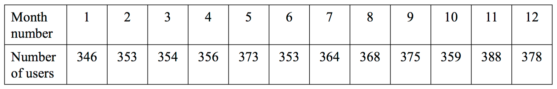
A four-point moving mean with centring is used to smooth timeline series.
The smoothed value of the number of users in month number 5 is closest to

A. `357`

B. `359`

C. `360`

D. `365`

E. `373`

Part 3

A least squares regression line is ﬁtted to the time series plot.
The equation of this least squares regression line is

number of users = 346 + 2.77 × month number

Let month number 1 = January 2007, month number 2 = February 2007, and so on.

Using the above information, the regression line predicts that the number of users in December 2009 will be closest to

A. `379`

B. `412`

C. `443`

D. `446`

E. `448`

Show Answers Only

`text(Part 1:)\ E`

`text(Part 2:)\ C`

`text(Part 3:)\ D`

Show Worked Solution

`text(Part 1)`

♦ Mean mark 39%.
MARKERS’ COMMENT: 50% of students incorrectly read the three large random fluctuations in monthly sales as seasonality, which can’t be determined over only 12 months.

`text(The time series is clearly trending upwards with)`

`text(higher lows and higher highs occurring.)`

`text(The large fluctuations are random and should)`

`text(not be confused with seasonality.)`

`=>E`

`text(Part 2)`

`text(Mean for months 3-6)`

`=(354+356+373+353)/4`

`=359`

`text(Mean for months 4-7)`

`=(356+373+353+364)/4`

`=361.5`

`:.\ text(Four point moving mean with centring)`

`=(359+361.5)/2`

`=360.25`

`=> C`

`text(Part 3)`

`text(December 2009 will be month number 36.)`

`:.\ text(Number of users)`	`= 346+2.77xx36`
	`= 445.72`

`=> D`

PATTERNS, FUR1 2013 VCAA 6 MC

There are 3000 tickets available for a concert.

On the first day of ticket sales, 200 tickets are sold.

On the second day, 250 tickets are sold.

On the third day, 300 tickets are sold.

This pattern of ticket sales continues until all 3000 tickets are sold.

How many days does it take for all of the tickets to be sold?

A. `5`

B. `6`

C. `8`

D. `34`

D. `57`

Show Answers Only

`C`

Show Worked Solution

`200+250+300+…`

`text(AP where)\ \ \ a`	`=200`
`d`	`=250-200=50`

`text(Find)\ n,\ text(when)\ S_n=3000`

`S_n`	`=n/2[2a+(n-1)d]`
`3000`	`=n/2[2×200+(n-1)50]`
	`=n/2(400+50n-50)`
	`=n/2(350+50n)`
`3000`	`=175n+25n^2`

`n^2+7n-120`	`=0`
`(n-8)(n+15)`	`=0`

`:. n=8,\ \ \ (n>0)`

`=> C`

CORE*, FUR1 2013 VCAA 5 MC

A sequence is generated by the difference equation

`t_(n+1)=2 xx t_n,\ \ \ \ \ t_1=1`

The `n`th term of this sequence is

A. `t_n=1×2^(n-1)`

B. `t_n=1+2^(n-1)`

C. `t_n=1+2×(n-1)`

D. `t_n=2+(n-1)`

E. `t_n=2+1^(n-1)`

Show Answers Only

`A`

Show Worked Solution

`t_2`	`=2 xx t_1 = 2`
`t_3`	`=2 xx t_2 = 2^2`
`t_4`	`=2 xx t_3 = 2^3`
`t_5`	`=2 xx t_4 = 2^4`

`vdots`

♦ Mean mark 48%.

`t_n= 1 xx 2^(n-1)`

`=> A`

CORE, FUR1 2013 VCAA 9 MC

The following data was recorded in an investigation of the relationship between age and reaction time. In this investigation, age is the explanatory variable.

Several statistics were calculated for this data.

When the data was checked, a recording error was found; the age of a 69-year-old had been incorrectly entered as 96. The recording error was corrected and the statistics were calculated.

The statistics that will remain unchanged when recalculated is the

A. slope of the three median line.

B. intercept of the least squares regression line.

C. correlation coefficient, `r`.

D. range of age.

E. standard deviation of age.

Show Answers Only

`A`

Show Worked Solution

`text(By elimination,)`

♦ Mean mark 47%.

`text(A change in value of an independent variable)`

`text(data point will effect)\ B, C,\ text(and)\ E.`

`text(Considering)\ D,`

`text(S)text(ince 96 was the high, changing it will change)`

`text(the range. Not)\ D.`

`text(Considering)\ A,`

`text{Upper group (4 highest ages) has the same median}`

`text(whether 96 or 69 is the high.)\ A\ text(will be unchanged.)`

`=> A`

CORE, FUR1 2013 VCAA 3-4 MC

The heights of 82 mothers and their eldest daughters are classified as 'short', 'medium' or 'tall'. The results are displayed in the frequency table below.

Part 1

The number of mothers whose height is classified as 'medium' is

A. `7`

B. `10`

C. `14`

D. `31`

E. `33`

Part 2

Of the mothers whose height is classified as 'tall', the percentage who have eldest daughters whose height is classified as 'short' is closest to

A. `text(3%)`

B. `text(4%)`

C. `text(14%)`

D. `text(17%)`

E. `text(27%)`

Show Answers Only

`text(Part 1:)\ D`

`text(Part 2:)\ C`

Show Worked Solution

`text(Part 1)`

`text(# Mothers classified as medium)`

`=10+14+7\ \ \ text{(from Table)}`

`=31`

`=>D`

`text(Part 2)`

♦ Mean mark 45%.
MARKER’S COMMENT: Many students obtained the wrong base of 82 for this percentage calculation.

`text(# Tall Mothers)`	`=3+11+8`
	`=22`

`text{# Tall Mothers with short eldest = 3 (from Table)}`

`:.\ text(Percentage)`	`=3/22×100`
	`=13.6363…%`

`=> C`

Quadratic, EXT1 2008 HSC 4c

The points `P(2ap, ap^2)`, `Q(2aq, aq^2)` lie on the parabola `x^2 = 4ay`. The tangents to the parabola at `P` and `Q` intersect at `T`. The chord `QO` produced meets `PT` at `K`, and `/_PKQ` is a right angle.

Find the gradient of `QO`, and hence show that `pq = –2`. (2 marks)
The chord `PO` produced meets `QT` at `L`. Show that `/_PLQ` is a right angle. (1 mark)
Let `M` be the midpoint of the chord `PQ`. By considering the quadrilateral `PQLK`, or otherwise, show that `MK = ML`. (2 marks)

Show Answers Only

`text(Proof)\ \ text{(See Worked Solutions)}`
`text(Proof)\ \ text{(See Worked Solutions)}`
`text(Proof)\ \ text{(See Worked Solutions)}`

Show Worked Solution

(i) `Q(2aq, aq^2),\ \ \ \ O(0,0)`

`m_(QO)`	`= (y_2 – y_1)/(x_2 – x_1)`
	`= (aq^2 – 0)/(2aq – 0)`
	`= q/2`

`text(Gradient of tangent at)\ P = p`

`text(We know the extension of chord)\ \ QO _|_ PT\ \ \ text{(given)}`

`m_(QO) xx m_(PT)`	`= -1`
`q/2 xx p`	`= -1`
`:. pq`	`= -2\ \ \ text(… as required.)`

(ii) `m_(PO) = (ap^2-0)/(2ap-0) = p/2`

`m\ text(of tangent)\ QT = q`

`m_(PO) xx m_(QT)`	`= p/2 xx q`
	`= (pq)/2`
	`= (-2)/2\ \ \ text{(from (i))}`
	`= -1`

`:.\ /_PLQ\ text(is a right angle.)`

(iii) `PQ\ text(subtends 2 right-angles at)\ L\ text(and)\ K`

`=>\ PQLK\ text(is a cyclic quad, with)\ \ PQ`

`text(a diameter.)`

`=> text(Midpoint of)\ PQ=M\ \ \ text{(centre of the circle)}`

`:.\ MK = ML\ \ text{(radii)}`

Combinatorics, EXT1 A1 2008 HSC 4b

Barbara and John and six other people go through a doorway one at a time.

In how many ways can the eight people go through the doorway if John goes through the doorway after Barbara with no-one in between? (1 mark)

--- 2 WORK AREA LINES (style=lined) ---
Find the number of ways in which the eight people can go through the doorway if John goes through the doorway after Barbara. (1 mark)

--- 6 WORK AREA LINES (style=lined) ---

Show Answers Only

`5040`
`20\ 160`

Show Worked Solution

i. `text(Barbara and John can be treated as one person)`

`:.\ text(# Combinations)`	`= 7!`
	`= 5040`

ii. `text(Solution 1)`

`text(Total possible combinations)=8!`

`text(Barbara has an equal chance of being behind as)`

`text(being in front of John.)`

`:.\ text{# Combinations (John before Barbara)}`

`=(8!)/2`

`=20\ 160`

`text(Solution 2)`

`text(If)\ B\ text(goes first,)\ J\ text(has 7 options and the other)`

`text(6 people can go in any order.)`

`=> text(# Combinations) = 7 xx 6!`

`text(If)\ B\ text(goes second,)\ J\ text(has 6 options)`

`=> text(# Combinations) = 6 xx 6!`

`text(If)\ B\ text(goes third,)\ J\ text(has 5 options)`

`=> text(# Combinations) = 5 xx 6!`

`text(And so on…)`

`:.\ text(Total Combinations)`

`= 7 xx 6! + 6 xx 6! + … + 1 xx 6!`

`= 6! ( 7 + 6 + 5 + 4 + 3 + 2 + 1)`

`= 6! ( 28)`

`= 20\ 160`

Calculus, EXT1 C1 2008 HSC 3c

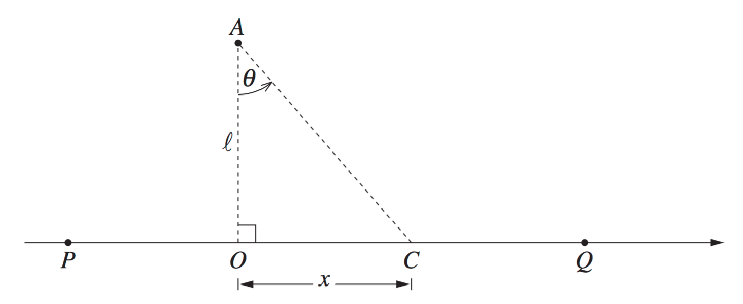
A race car is travelling on the `x`-axis from `P` to `Q` at a constant velocity, `v`.

A spectator is at `A` which is directly opposite `O`, and `OA = l` metres. When the car is at `C`, its displacement from `O` is `x` metres and `/_OAC = theta`, with `- pi/2 < theta < pi/2`.

Show that `(d theta)/(dt) = (vl)/(l^2 + x^2)`. (2 marks)

--- 8 WORK AREA LINES (style=lined) ---
Let `m` be the maximum value of `(d theta)/dt`.

Find the value of `m` in terms of `v` and `l`. (1 mark)

--- 2 WORK AREA LINES (style=lined) ---
There are two values of `theta` for which `(d theta)/(dt) = m/4`.

Find these two values of `theta`. (2 marks)

--- 6 WORK AREA LINES (style=lined) ---

Show Answers Only

`text(Proof)\ \ text{(See Worked Solutions)}`
`v/l`
`+- pi/3`

Show Worked Solution

i. `text(Show)\ \ (d theta)/(dt) = (vl)/(l^2 + x^2)`

`(d theta)/(dt)`	`= (d theta)/(dx) * (dx)/(dt)\ \ \ \ \ \ \ …\ (1)`
`v`	`= (dx)/(dt)\ \ \ text{(given)}`

`text(Find)\ \ (d theta)/(dx),`

MARKER’S COMMENT: The most successful students used `theta=tan^-1(x/l)` and the chain rule to find `(d theta)/(dt)`.

`tan theta`	`= x/l`
`theta`	`= tan^-1 (x/l)`
`(d theta)/(dx)`	`= l/(l^2+x^2)`

`text{Substituting into (1),}`
`(d theta)/(dt)`	`= l/(l^2+x^2) * v`
	`= (vl)/(l^2 + x^2)\ \ \ text(… as required)`

ii. `(d theta)/(dt)\ \ text(is a MAX when)\ \ x = 0`

`:. m`	`= (vl)/(l^2 + 0^2)`
	`= v/l`

iii. `text(Find)\ \ theta\ \ text(when)\ \ (d theta)/(dt) = m/4`

MARKER’S COMMENT: Many students lost marks by not giving their answer in the specified range. Be careful!

`=> (d theta)/(dt)`	`= v/(4l)`
`(vl)/(l^2 +x^2)`	`= v/(4l)`
`l^2 + x^2`	`= 4l^2`
`x^2`	`= 3l^2`
`x`	`= +- sqrt3 l`

`tan theta`	`= x/l`
	`= +- sqrt 3`
`:. theta`	`= +- pi/3,\ \ \ \ \ (- pi/2 < theta < pi/2)`

Financial Maths, STD2 F5 SM-Bank 3

Camilla buys a car for $21 000 and repays it over 4 years through equal monthly instalments.

She pays a 10% deposit and interest is charged at 9% p.a. on the reducing balance loan.

Using the Table of present value interest factors below, where `r` represents the monthly interest and `N` represents the number of repayments

Calculate the monthly repayment, `$P`, that Camilla must pay to complete the loan after 4 years (to the nearest $). (3 marks)

--- 6 WORK AREA LINES (style=lined) ---
Calculate the total interest paid over the life of the loan. (1 mark)

--- 1 WORK AREA LINES (style=lined) ---

Show Answers Only

`text(Camilla must repay $470 per month)`
`$3660`

Show Worked Solution

i. `text(Deposit) = 10text(%) xx 21\ 000 = 2100`

`text(Loan Value)`	`= 21\ 000 – 2100`
	`= 18\ 900`

`text(Monthly interest rate) = text(9%)/12 = 0.0075`

`text(# Repayments) = 4 xx 12 = 48`

`=>\ text(PVA Factor) = 40.18478\ \ text{(from Table)}`

`text(Monthly repayment)\ ($P)`	`= (18\ 900)/(40.18478)`
	`= 470.32…`
	`= 470\ text{(nearest $)}`

`:.\ text(Camilla must repay $470 per month.)`

ii. `text(Total Repayments)`

`= 48 xx 470`

`= $22\ 560`

`:.\ text(Interest paid over loan)`

`= 22\ 560 – 18\ 900`

`= $3660`

Polynomials, EXT1 2008 HSC 2d

The function `f(x) = tan x − log_e x` has a zero near `x = 4`.

Use one application of Newton’s method to obtain another approximation to this zero. Give your answer correct to two decimal places. (3 marks)

Show Answers Only

`4.11\ \ text{(2 d.p.)}`

Show Worked Solution

`f(x)`	`= tanx – log_ex`
`f'(x)`	`= sec^2x – 1/x`

`text(Zero near)\ \ x = 4`

`f(4)`	`= tan 4 – log_e 4`
	`= -0.2284…`
`f'(4)`	`= sec^2 4 – 1/4`
	`= 2.0905…`

`x_1`	`= x_0 – f(4)/(f'(4))`
	`= 4 – ((-0.2284…))/(2.0905…)`
	`= 4.109…`
	`= 4.11\ \ text{(2 d.p.)}`

Statistics, STD2 S5 2008 HSC 28a

The following graph indicates `z`-scores of ‘height-for-age’ for girls aged 5 – 19 years.

What is the `z`-score for a six year old girl of height 120 cm? (1 mark)

--- 2 WORK AREA LINES (style=lined) ---
Rachel is 10 ½ years of age.

(1) If 2.5% of girls of the same age are taller than Rachel, how tall is she? (1 mark)

--- 1 WORK AREA LINES (style=lined) ---

(2) Rachel does not grow any taller. At age 15 ½, what percentage of girls of the same age will be taller than Rachel? (2 marks)

--- 4 WORK AREA LINES (style=lined) ---
What is the average height of an 18 year old girl? (1 mark)

--- 1 WORK AREA LINES (style=lined) ---

For adults (18 years and older), the Body Mass Index is given by

`B = m/h^2` where `m = text(mass)` in kilograms and `h = text(height)` in metres.

The medically accepted healthy range for `B` is `21 <= B <= 25`.

What is the minimum weight for an 18 year old girl of average height to be considered healthy? (2 marks)

--- 4 WORK AREA LINES (style=lined) ---
The average height, `C`, in centimetres, of a girl between the ages of 6 years and 11 years can be represented by a line with equation

`C = 6A + 79` where `A` is the age in years.

(1) For this line, the gradient is 6. What does this indicate about the heights of girls aged 6 to 11? (1 mark)

--- 2 WORK AREA LINES (style=lined) ---

(2) Give ONE reason why this equation is not suitable for predicting heights of girls older than 12. (1 mark)

--- 2 WORK AREA LINES (style=lined) ---

Show Answers Only

`1`
(1) `155\ text(cm)`

(2) `text(84%)`
`163\ text(cm)`
`55.8\ text(kg)`
(1) `text(It indicates that 6-11 year old girls)`

`text(grow, on average, 6cm per year)`

(2) `text(Girls eventually stop growing, and the)`

`text(equation doesn’t factor this in.)`

Show Worked Solution

i.	`z text(-score) = 1`

ii.	(1)	`text(If 2 ½ % are taller than Rachel)`
		`=> z text(-score of +2)`
		`:.\ text(She is 155 cm)`

	(2)	`text(At age)\ 15\ ½,\ 155\ text(cm has a)\ z text(-score of –1)`
		`text(68% between)\ z = 1\ text(and)\ –1`
		`=> text(34% between)\ z = 0\ text(and)\ –1`
		`text(50% have)\ z >= 0`

		`:.\ text(% Above)\ z text(-score of –1)`
		`= 50 + 34`
		`= 8text(4%)`

`:.\ text(84% of girls would be taller than Rachel at age)\ 15 ½.`

iii.	`text(Average height of 18 year old has)\ z text(-score = 0)`
	`:.\ text(Average height) = 163\ text(cm)`

iv.	`B = m/h^2`
	`h = 163\ text(cm) = 1.63\ text(m)`

`text(Given)\ \ 21 <= B <= 25,\ text(minimum healthy)`

`text(weight occurs when)\ B = 21`

`=> 21`	`= m/1.63^2`
`m`	`= 21 xx 1.63^2`
	`= 55.794…`
	`= 55.8\ text(kg)\ text{(1 d.p.)}`

v.	(1)	`text(It indicates that 6-11 year old girls, on average, grow)`
		`text(6 cm per year.)`
	(2)	`text(Girls eventually stop growing, and the equation doesn’t)`
		`text(factor this in.)`

Statistics, STD2 S1 2008 HSC 26d

The graph shows the predicted population age distribution in Australia in 2008.

How many females are in the 0–4 age group? (1 mark)

--- 1 WORK AREA LINES (style=lined) ---
What is the modal age group? (1 mark)

--- 1 WORK AREA LINES (style=lined) ---
How many people are in the 15–19 age group? (2 marks)

--- 4 WORK AREA LINES (style=lined) ---
Give ONE reason why there are more people in the 80+ age group than in the 75–79 age group. (1 mark)

--- 2 WORK AREA LINES (style=lined) ---

Show Answers Only

`600\ 000`
`35-39`
`1\ 450\ 000`
`text(The 80+ group includes all people over 80)`
`text(and is not restricted by a 5-year limit.)`

Show Worked Solution

a.	`text{# Females (0-4)}`	`= 0.6 xx 1\ 000\ 000`
		`= 600\ 000`

`text(Modal age group)\ =`

`text(35 – 39)`

c.	`text{# Males (15-19)}`	`= 0.75 xx 1\ 000\ 000`
		`= 750\ 000`

`text{# Females (15-19)}`	`= 0.7 xx 1\ 000\ 000`
	`= 700\ 000`

`:.\ text{Total People (15-19)}`	`= 750\ 000 + 700\ 000`
	`= 1\ 450\ 000`

d.	`text(The 80+ group includes all people over 80)`
	`text(and is not restricted by a 5-year limit.)`

Probability, 2UG 2008 HSC 26c

Joel is designing a game with four possible outcomes. He has decided on three of these outcomes.

What must be the value of the loss in Outcome 4 in order for the financial expectation of this game to be $0? (2 marks)

Show Answers Only

`$22.50`

Show Worked Solution

`text(Chance of outcome 4)`

`= 100 – (10 + 40 + 30)`

`= 20text(%)`

`text(Let)\ \ X = text(Loss from Outcome 4)`

`text(We know Fin Exp = 0)`

`=> 0`	`= (0.1 xx 12) + (0.4 xx 6) + (0.3 xx 3) – 0.2X`
`0.2X`	`= 1.2 + 2.4 + 0.9`
	`= 4.5`
`X`	`= $22.5`

`:.\ text(The loss in outcome 4 must be $22.50.)`

Probability, STD2 S2 2008 HSC 26b

The retirement ages of two million people are displayed in a table.

What is the relative frequency of the 51–55 year retirement age? (1 mark)

--- 1 WORK AREA LINES (style=lined) ---
Describe the distribution. (1 mark)

--- 2 WORK AREA LINES (style=lined) ---

Show Answers Only

`7/400`
`text(Distribution is negatively skewed because)`

`text(as age increases, so does the number of)`

`text(people in each age bracket.)`

Show Worked Solution

i. `text(Relative frequency)\ (51-55)`

`= text{# People (51-55)}/text(Total People)`

`= (35\ 000)/(2\ 000\ 000)`

`= 7/400`

ii. `text(Distribution is negatively skewed because)`

`text(as age increases, so does the number of)`

`text(people in each age bracket.)`

Measurement, STD2 M6 2008 HSC 25c

Pieces of cheese are cut from cylindrical blocks with dimensions as shown.

Twelve pieces are packed in a rectangular box. There are three rows with four pieces of cheese in each row. The curved surface is face down with the pieces touching as shown.

What are the dimensions of the rectangular box? (4 marks)

--- 8 WORK AREA LINES (style=lined) ---

To save packing space, the curved section is removed.
What is the volume of the remaining triangular prism of cheese? Answer to the nearest cubic centimetre. (2 marks)

--- 4 WORK AREA LINES (style=lined) ---

Show Answers Only

`41\ text(cm) xx 21\ text(cm) xx 15\ text(cm)`
`506\ text(cm)³\ text{(nearest whole)}`

Show Worked Solution

a. `text(Box height) = 15\ text(cm)`

♦ Mean mark 45%.

`text{(radius of the arc)}`

`text(Box width)`	`= 3 xx 7`
	`= 21\ text(cm)`
`text(Box length)`	`= 4x`

`text(Using cosine rule)`

`c^2`	`= a^2 + b^2 – 2ab cos C`
`x^2`	`= 15^2 + 15^2 – 2 xx 15 xx 15 xx cos 40^@`
	`= 450 – 344.7199…`
	`= 105.2800…`
`x`	`= 10.2606…`

`text(Box length)`	`= 4 xx 10.2606…`
	`= 41.04…`

`:.\ text(Dimensions are)\ \ 41\ text(cm) xx 21\ text(cm) xx 15\ text(cm)`

b. `text(Volume) = Ah`

♦♦♦ Mean mark 22%.

`h = 7\ text(cm)`

`text(Find)\ A:`

`A`	`= 1/2 ab sin C`
	`= 1/2 xx 15 xx 15 xx sin 40^@`
	`= 72.3136…`

`:. V`	`= 72.3136… xx 7`
	`= 506.195…`
	`= 506\ text(cm³)\ \ text{(nearest whole)}`

Probability, STD2 S2 2008 HSC 25b

In a drawer there are 30 ribbons. Twelve are blue and eighteen are red.

Two ribbons are selected at random.

Copy and complete the probability tree diagram. (1 mark)
What is the probability of selecting a pair of ribbons which are the same colour? (2 marks)

--- 4 WORK AREA LINES (style=lined) ---

Show Answers Only

`73/145`

Show Worked Solution

ii. `Ptext{(same colour)}`

`=\ text{P(BB) + P(RR)}`

`= 12/30 xx 11/29 + 18/30 xx 17/29`

`= 132/870 + 306/870`

`= 73/145`

Probability, STD2 S2 2008 HSC 24b

Three-digit numbers are formed from five cards labelled 1, 2, 3, 4 and 5.

How many different three-digit numbers can be formed? (1 mark)

--- 1 WORK AREA LINES (style=lined) ---
If one of these numbers is selected at random, what is the probability that it is odd? (1 mark)

--- 2 WORK AREA LINES (style=lined) ---
How many of these three-digit numbers are even? (1 mark)

--- 2 WORK AREA LINES (style=lined) ---
What is the probability of randomly selecting a three-digit number less than 500 with its digits arranged in descending order? (2 marks)

--- 4 WORK AREA LINES (style=lined) ---

Show Answers Only

`60`
`3/5`
`24`
`1/15`

Show Worked Solution

i. `text(# Different numbers)`

♦ Mean mark 45%.

`= 5 xx 4 xx 3`

`= 60`

ii. `text(The last digit must be one of the)`

`text(5 numbers, of which 3 are odd)`

`:.\ text{P(odd)} = 3/5`

iii. `text{P(even)} = 1- text{P(odd)} = 2/5`

♦ Mean mark 48%.

`:.\ text(Number of even numbers)`

`= 2/5 xx 60`

`= 24`

iv. `text(The numbers that satisfy the criteria:)`

♦♦♦ Mean mark 10%.

`432, 431, 421, 321`

`:.\ text{P(selection)} = 4/60 = 1/15`

Statistics, STD2 S1 2008 HSC 23f

Christina has completed three Mathematics tests. Her mean mark is 72%.

What mark (out of 100) does she have to get in her next test to increase her mean mark to 73%? (2 marks)

--- 5 WORK AREA LINES (style=lined) ---

Show Answers Only

`76`

Show Worked Solution

`text(Total marks in 3 tests)`

`= 3 xx 72`

`= 216`

`text(We need 4-test mean) = 73`

`text(i.e.)\ \ \ `	`text{Total Marks (4 tests)}-:4`	`= 73`
	`text(Total Marks)\ text{(4 tests)}`	`= 292`

`:.\ text(4th test score)`	`= 292 – 216`
	`= 76`

Probability, STD2 S2 2008 HSC 22 MC

A die has faces numbered 1 to 6. The die is biased so that the number 6 will appear more often than each of the other numbers. The numbers 1 to 5 are equally likely to occur.

The die was rolled 1200 times and it was noted that the 6 appeared 450 times.

Which statement is correct?

The probability of rolling the number 5 is expected to be `1/7`.
The number 6 is expected to appear 2 times as often as any other number.
The number 6 is expected to appear 3 times as often as any other number.
The probability of rolling an even number is expected to be equal to the probability of rolling an odd number.

Show Answers Only

`C`

Show Worked Solution

`P(6) = 450/1200 = 3/8`

`text(Numbers 1-5 are rolled) = 1200-450=750\ text(times)`

`:.\ text(Each number is expected to appear)`

`750/5 = 150\ text(times)`

`:.P text{(specific number ≠ 6)}`

`= 150/1200`

`= 1/8`

`=> C`

Probability, STD2 S2 2008 HSC 18 MC

New car registration plates contain two letters followed by two numerals followed by two more letters eg AC 12 DC. Letters and numerals may be repeated.

Which of the following expressions gives the correct number of car registration plates that begin with the letter M?

`26^3 xx 10^2`
`25^3 xx 10^2`
`26^4 xx 10^2`
`25^4 xx 10^2 `

Show Answers Only

`A`

Show Worked Solution

`text(# Plates beginning with M)`

`= 1 xx 26 xx 10 xx 10 xx 26 xx 26`

`= 26^3 xx 10^2`

`=> A`

Measurement, STD2 M6 2008 HSC 17 MC

The diagram shows the position of `Q`, `R` and `T` relative to `P`.

In the diagram,

`Q` is south-west of `P`

`R` is north-west of `P`

`/_QPT` is 165°

What is the bearing of `T` from `P`?

`060^@`
`075^@`
`105^@`
`120^@`

Show Answers Only

`A`

Show Worked Solution

`/_QPS=45^@\ \ \ text{(} Q\ text(is south west of)\ Ptext{)}`

`/_TPS = 165 – 45 = 120^@`

`:.\ /_NPT = 60^@\ \ text{(} 180^@\ text(in straight line) text{)}`

`=> A`

Calculus, 2ADV C4 2008 HSC 10a

In the diagram, the shaded region is bounded by `y = log_e (x – 2)`, the `x`-axis and the line `x = 7`.

Find the exact value of the area of the shaded region. (5 marks)

Show Answers Only

`5 log_e 5 – 4\ \ \ text(u²)`

Show Worked Solution

`text(Shaded Area)\ text{(} A_1 text{)}`	`=\ text(Rectangle) – A_2`
`text(Area of Rectangle)\ `	`= 7 xx log_e 5`

`text(Finding the Area of)\ \ A_2`

`y`	`= log_e (x – 2)`
`x – 2`	`= e^y`
`x`	`= e^y + 2`

`:. A_2`	`= int_0^(log_e 5) x\ dy`
	`= int_0^(log_e 5) e^y + 2\ dy`
	`= [e^y + 2y]_0^(log_e 5)`
	`= [(e^(log_e 5) + 2 log_e 5) – (e^0 + 0)]`
	`= (5 + 2 log_e 5) – 1`
	`= 4 + 2 log_e 5`

`:.\ A_1`	`= 7 log_e 5 – (4 + 2 log_e 5)`
	`= 5 log_e 5 – 4\ \ \ text(u²)`

Calculus, 2ADV C4 2008 HSC 9c

A beam is supported at `(-b, 0)` and `(b, 0)` as shown in the diagram.

It is known that the shape formed by the beam has equation `y = f(x)`, where `f(x)` satisfies

	`f^{″}(x)`	`= k (b^2-x^2),\ \ \ \ \ `(`k` is a positive constant)
and	`f^{′}(-b)`	`= -f'(b)`.

Show that `f^{′}(x) = k (b^2x-(x^3)/3)`. (2 marks)

--- 5 WORK AREA LINES (style=lined) ---
How far is the beam below the `x`-axis at `x = 0`? (2 marks)

--- 6 WORK AREA LINES (style=lined) ---

Show Answers Only

`text(Proof)\ text{(See Worked Solutions)}`
`(5kb^4)/12\ text(units)`

Show Worked Solution

i.	`text(Show)\ \ f^{′}(x) = k (b^2x-x^3/3)`

`f^{″}(x)`	`= k (b^2 – x^2)`
`f^{′}(x)`	`= int k (b^2-x^2)\ dx`
	`= k int b^2-x^2\ dx`
	`= k (b^2x-x^3/3) + c`

`text(S)text(ince S.P. exists at)\ \ x = 0`

`=> f^{′}(x)`	`= 0\ \ text(when)\ \ x = 0`
`0`	`= k (b^2 * 0-0) + c`
`c`	`= 0`

`:.\ f^{′}(x) = k (b^2x-x^3/3)\ \ \ text(… as required)`

ii.	`f(x)`	`= int f^{′}(x)\ dx`
		`= k int b^2x-x^3/3\ dx`
		`= k ((b^2x^2)/2-x^4/12) + c`

`text(We know)\ \ f(x) = 0\ \ text(when)\ \ x = b`

`=> 0`	`= k ( (b^2*b^2)/2-b^4/12) + c`
`c`	`= -k ( (6b^4)/12-b^4/12)`
	`= -k ( (5b^4)/12 )`
	`= -(5kb^4)/12`

`:.\ text(When)\ \ x = 0, text(the beam is)\ \ (5kb^4)/12\ \ text(units)`

`text(below the)\ x text(-axis.)`

Probability, 2ADV S1 2008 HSC 9a

It is estimated that 85% of students in Australia own a mobile phone.

Two students are selected at random. What is the probability that neither of them owns a mobile phone? (2 marks)

--- 4 WORK AREA LINES (style=lined) ---
Based on a recent survey, 20% of the students who own a mobile phone have used their mobile phone during class time. A student is selected at random. What is the probability that the student owns a mobile phone and has used it during class time? (1 mark)

--- 2 WORK AREA LINES (style=lined) ---

Show Answers Only

`9/400`
`17/100`

Show Worked Solution

i. `P(M) = 0.85`

COMMENT: `M^c` is syllabus notation for the complement of event `M`.

`P(M^c) = 1-0.85 = 0.15`

`:.\ P(M^c, M^c)`	`= 15/100 * 15/100`
	`= 225/(10\ 000)`
	`= 9/400`

ii. `text{P(owns mobile and used it)}`

`= P(M) xx P\text{(used it)}`

`= 17/20 xx 20/100`

`= 17/100`

Plane Geometry, 2UA 2008 HSC 8b

In the diagram, `ABCD` is a parallelogram and `ABEF` and `BCGH` are both squares.

Copy or trace the diagram into your writing booklet.

Prove that `CD = BE`. (1 mark)
Prove that `BD = EH`. (3 marks)

Show Answers Only

`text(Proof)\ \ text{(See Worked Solutions)}`
`text(Proof)\ \ text{(See Worked Solutions)}`

Show Worked Solution

(i) `text(Prove)\ CD = BE`

`CD`	`= AB\ \ text{(opposite sides of parallelogram)}`
`AB`	`= BE\ \ text{(sides of square)}`
`:.\ CD`	`= BE\ \ \ text(… as required)`

(ii)

`text(Prove)\ BD = EH`

`CD`	`= BE\ \ text{(from part (i))}`
`BC`	`= BH\ \ text{(sides of square)}`

`/_BDC = /_ABD = alpha\ \ text{(} text(alternate,)\ AB\ text(||)\ CD text{)}`

`text(Let)\ /_DBC = beta`

`/_BCD`	`= 180 – alpha – beta\ \ \ \ text{(angle sum of}\ Delta BDCtext{)}`
`/_EBH`	`= 360 – 90 – 90 – alpha – beta\ \ \ `
	`text{(angles about a point)}`
	`= 180 – alpha – beta`
	`= /_BCD`

`=> Delta DCB ~= Delta EBH\ \ text{(SAS)}`

`:.\ BD = EH\ \ \ `	`text{(corresponding sides of)`
	`\ \ text{congruent triangles)}`

Calculus, 2ADV C3 2008 HSC 8a

Let `f(x) = x^4 − 8x^2`.

Find the coordinates of the points where the graph of `y = f(x)` crosses the axes. (2 marks)

--- 5 WORK AREA LINES (style=lined) ---
Show that `f(x)` is an even function. (1 mark)

--- 2 WORK AREA LINES (style=lined) ---
Find the coordinates of the stationary points of `f(x)` and determine their nature. (4 marks)

--- 8 WORK AREA LINES (style=lined) ---
Sketch the graph of `y = f(x)`. (1 mark)

--- 8 WORK AREA LINES (style=lined) ---

Show Answers Only

`(-2 sqrt 2,0), (2 sqrt 2, 0)`
`text(Proof)\ \ text{(See Worked Solutions)}`
`text(S.P.s at)\ (0,0), (2,-16), (-2,-16)`

Show Worked Solution

i.	`f(x) = x^4 – 8x^2`

`y text(-intercept when)\ x = 0`

`:.\ text(Cuts)\ y\ text(axis at)\ (0,0)`

`x\ text(-intercept when)\ f(x) = 0`

`x^4 – 8x^2`	`= 0`
`x^2 (x^2 – 8)`	`= 0`

`x^2 – 8 = 0\ \ \ \ \ text(or)\ \ \ \ \ x = 0`

`x^2`	`= 8`
`x`	`= +- sqrt 8 = +- 2 sqrt 2`

`:.\ text(Cuts)\ x text(-axis at)\ (-2 sqrt 2,0),\ \ text(and)\ \ (2 sqrt 2, 0)`

`text{(Note that it only touches}\ xtext{-axis at (0,0))}`

ii.	`f(x)`	`= x^4 – 8x^2`
	`f(–x)`	`= (–x)^4 – 8(–x)^2`
		`= x^4 – 8x^2`
		`= f(x)`

`:.\ f(x)\ text(is an even function.)`

iii.	`f(x)`	`= x^4 – 8x^2`
	`f'(x)`	`= 4x^3 – 16x`
	`f″(x)`	`=12x^2-16`

`text(S.P. when)\ \ f'(x) = 0`

`4x^3 – 16x`	`= 0`
`4x (x^2 – 4)`	`= 0`

`x^2 – 4`	`=0\ \ \ \ \ x = 0`
`x^2`	`= 4`
`x`	`= +-2`

`text(At)\ x=2\ \ `	`f(x)`	`=(2)^4 – 8(2)^2 = -16`
	`f″(x)`	`=12(2^2)-16>0`

`:.\ text{MIN at (2, –16)}`

`:.\ text{MIN at (–2, –16)},\ \ \ (f(x)\ text(is even))`

`text(At)\ x=0\ \ `	`f(x)`	`=(0)^4 – 8(0)^2 = 0`
	`f″(x)`	`=12(0^2)-16<0`

`:.\ text{MAX at (0,0)}`

iv.

Probability, 2ADV S1 2008 HSC 7c

Xena and Gabrielle compete in a series of games. The series finishes when one player has won two games. In any game, the probability that Xena wins is `2/3` and the probability that Gabrielle wins is `1/3`.

Part of the tree diagram for this series of games is shown.

Complete the tree diagram showing the possible outcomes. (1 mark)
What is the probability that Gabrielle wins the series? (2 marks)

--- 4 WORK AREA LINES (style=lined) ---
What is the probability that three games are played in the series? (2 marks)

--- 4 WORK AREA LINES (style=lined) ---

Show Answers Only

`7/27`
`4/9`

Show Worked Solution

MARKER’S COMMENT: A tree diagram with 8 outcomes is incorrect (i.e. no third game is played if 1 player wins the first 2 games). If outcomes cannot occur, do not draw them on a tree diagram.

ii. `P text{(} G\ text(wins) text{)}`

`= P(XGG) + P (GXG) + P (GG)`

`= 2/3 * 1/3 * 1/3 + 1/3 * 2/3 * 1/3 + 1/3 * 1/3`

`= 2/27 + 2/27 + 1/9`

`= 7/27`

iii. `text(Method 1:)`

`P text{(3 games played)}`

`= P (XG) + P(GX)`

`= 2/3 * 1/3 + 1/3 * 2/3`

`= 4/9`

`text(Method 2:)`

`P text{(3 games)}`

`= 1 – [P(XX) + P(GG)]`

`= 1 – [2/3 * 2/3 + 1/3 * 1/3]`

`= 1 – 5/9`

`= 4/9`

Trigonometry, 2ADV T1 2008 HSC 7b

The diagram shows a sector with radius `r` and angle `theta` where `0 < theta <= 2pi`.

The arc length is `(10pi)/3`.

Show that `r >= 5/3`. (2 marks)

--- 4 WORK AREA LINES (style=lined) ---
Calculate the area of the sector when `r = 4`. (2 marks)

--- 3 WORK AREA LINES (style=lined) ---

Show Answers Only

`text(Proof)\ \ text{(See Worked Solutions)}`
`(20pi)/3\ text(u²)`

Show Worked Solution

i.	`text(Show)\ r >= 5/3`

`text(Arc length)\ `	`= r theta\ \ text(where)\ \ 0 < theta <= 2pi`
`r theta`	`= (10pi)/3`
`:.theta`	`= (10pi)/(3r)`

`text(Using)\ \ \ 0 <= theta <= 2 pi`

`0 <= (10pi)/(3r)`	`<= 2pi`
`(10pi)/3`	`<= 2 pi r`
`5/3`	`<= r`

`:.\ r >= 5/3\ \ \ text(… as required.)`

ii.	`text(Area)`	`= 1/2 r^2 theta`
		`= 1/2 xx 4^2 xx (10pi)/(3 xx 4)`
		`= (20pi)/3\ text(u²)`

Trigonometry, 2ADV T2 2008 HSC 6a

Solve `2 sin^2 (x/3) = 1` for `-pi <= x <= pi`. (3 marks)

--- 6 WORK AREA LINES (style=lined) ---

Show Answers Only

`x = -(3pi)/4, (3pi)/4`

Show Worked Solution

♦♦ Although exact data not available, markers specifically mentioned this question was poorly answered.

`2 sin^2 (x/3)`	`= 1\ \ text(for)\ \ -pi <= x <= pi`
`sin^2 (x/3)`	`= 1/2`
`sin (x/3)`	`= +- 1/sqrt2`

MARKER’S COMMENT: Many students had problems adjusting their answer to the given domain, especially when dealing with negative angles.

`text(When)\ sin (x/3) = 1/sqrt2`

`x/3`	`= pi/4, (3pi)/4`
`x`	`= (3pi)/4, (9pi)/4`

`text(When)\ sin (x/3) = – 1/sqrt2`

`x/3`	`= – pi/4, -(3pi)/4`
`x`	`= -(3pi)/4, -(9pi)/4`

`:.\ x = -(3pi)/4\ \ text(or)\ \ (3pi)/4\ \ text(for)\ \ -pi <= x <= pi`

Quadratic, 2UA 2008 HSC 4c

Consider the parabola `x^2 = 8(y\ – 3)`.

Write down the coordinates of the vertex. (1 mark)
Find the coordinates of the focus. (1 mark)
Sketch the parabola. (1 mark)
Calculate the area bounded by the parabola and the line `y = 5`. (3 marks)

Show Answers Only

(i) `(0,3)`

(ii) `(0,5)`

(iii)

(iv) `10 2/3\ text(u²)`

Show Worked Solution

(i)

`text(Vertex)\ = (0,3)`

(ii)	`text(Using)\ \ \ x^2`	`= 4ay`
	`4a`	`= 8`
	`a`	`= 2`

`:.\ text(Focus) = (0,5)`

(iii)

(iv)

`text(Intersection when)\ y = 5`

`=> x^2`	`= 8 (5-3)`
`x^2`	`= 16`
`x`	`= +- 4`

`text(Find shaded area)`

`x^2`	`= 8 (y-3)`
`y – 3`	`= x^2/8`
`y`	`= x^2/8 +3`

`text(Area)`	`= int_-4^4 5\ dx – int_-4^4 x^2/8 + 3\ dx`
	`= int_-4^4 5 – (x^2/8 + 3)\ dx`
	`= int_-4^4 2 – x^2/8\ dx`
	`= [2x – x^3/24]_-4^4`
	`= [(8 – 64/24) – (-8 + 64/24)]`
	`= 5 1/3 – (- 5 1/3)`
	`= 10 2/3\ text(u²)`

Mechanics, EXT2* M1 2014 HSC 14a

The take-off point `O` on a ski jump is located at the top of a downslope. The angle between the downslope and the horizontal is `pi/4`. A skier takes off from `O` with velocity `V` m s⁻¹ at an angle `theta` to the horizontal, where `0 <= theta < pi/2`. The skier lands on the downslope at some point `P`, a distance `D` metres from `O`.

The flight path of the skier is given by

`x = Vtcos theta,\ y = -1/2 g t^2 + Vt sin theta`, (Do NOT prove this.)

where `t` is the time in seconds after take-off.

Show that the cartesian equation of the flight path of the skier is given by

`y = x tan theta - (gx^2)/(2V^2) sec^2 theta`. (2 marks)

--- 5 WORK AREA LINES (style=lined) ---
Show that

`D = 2 sqrt 2 (V^2)/(g) cos theta (cos theta + sin theta)`. (3 marks)

--- 8 WORK AREA LINES (style=lined) ---
Show that

`(dD)/(d theta) = 2 sqrt 2 (V^2)/(g) (cos 2 theta - sin 2 theta)`. (2 marks)

--- 4 WORK AREA LINES (style=lined) ---
Show that `D` has a maximum value and find the value of `theta` for which this occurs. (3 marks)

--- 9 WORK AREA LINES (style=lined) ---

Show Answers Only

`text(Proof)\ \ text{(See Worked Solutions)}`
`text(Proof)\ \ text{(See Worked Solutions)}`
`text(Proof)\ \ text{(See Worked Solutions)}`
`text(Proof)\ \ text{(See Worked Solutions)}`

Show Worked Solution

i. `text(Show)\ \ y = x tan theta – (gx^2)/(2V^2) sec^2 theta`

`x`	`= Vt cos theta`
`t`	`= x/(V cos theta)\ \ \ …\ text{(1)}`

`text(Subst)\ text{(1)}\ text(into)\ y = -1/2 g t^2 + Vt sin theta`

`y`	`= -1/2 g (x/(Vcostheta))^2 + V sin theta (x/(Vcostheta))`
	`= (-gx^2)/(2V^2 cos^2 theta) + x * (sin theta)/(cos theta)`
	`= x tan theta – (gx^2)/(2V^2) sec^2 theta\ \ \ text(… as required.)`

ii. `text(Show)\ D = 2 sqrt 2 (V^2)/g\ cos theta (cos theta + sin theta)`

♦♦ Mean mark 28%
MARKER’S COMMENT: The key to finding `P` and solving for `D` is to realise you need the intersection of the Cartesian equation in (i) and the line `y=–x`.

`text(S)text(ince)\ P\ text(lies on line)\ y = -x`

`-x`	`=x tan theta – (gx^2)/(2V^2) sec^2 theta`
`-1`	`=tan theta – (gx)/(2V^2) sec^2 theta`
`(gx)/(2V^2) sec^2 theta`	`= tan theta + 1`
`x (g/(2V^2))`	`=(sin theta)/(cos theta) * cos^2 theta + 1 * cos^2 theta`
`x`	`=(2V^2)/g\ (sin theta cos theta + cos^2 theta)`
	`=(2V^2)/g\ cos theta (cos theta + sin theta)`

`text(Given that)\ \ cos(pi/4)`	`= x/D = 1/sqrt2`
`text(i.e.)\ \ D`	`= sqrt 2 x`

`:.\ D = 2 sqrt 2 (V^2)/g\ cos theta (cos theta + sin theta)`

`text(… as required.)`

iii. `text(Show)\ (dD)/(d theta) = 2 sqrt 2 (V^2)/g\ (cos 2 theta – sin 2 theta)`

`D`	`= 2 sqrt 2 (V^2)/g\ (cos^2 theta + cos theta sin theta)`
`(dD)/(d theta)`	`= 2 sqrt 2 (V^2)/g\ [2cos theta (–sin theta) + cos theta cos theta + (– sin theta) sin theta]`
	`= 2 sqrt 2 (V^2)/(g) [(cos^2 theta – sin^2 theta) – 2 sin theta cos theta]`
	`= 2 sqrt 2 (V^2)/g\ (cos 2 theta – sin 2 theta)\ \ \ text(… as required)`

iv. `text(Max/min when)\ (dD)/(d theta) = 0`

♦ Mean mark 47%
IMPORTANT: Note that students can attempt every part of this question, even if they couldn’t successfully prove earlier parts.

`2 sqrt 2 (V^2)/g\ (cos 2 theta – sin 2 theta)`	`= 0`
`cos 2 theta – sin 2 theta`	`= 0`
`sin 2 theta`	`= cos 2 theta`
`tan 2 theta`	`= 1`
`2 theta`	`= pi/4`
`theta`	`= pi/8`

`(d^2D)/(d theta^2)`	`= 2 sqrt 2 (V^2)/g\ [-2 sin 2theta – 2 cos 2 theta]`
	`= 4 sqrt 2 (V^2)/g\ (-sin 2 theta – cos 2 theta)`

`text(When)\ \ theta = pi/8:`

`(d^2 D)/(d theta^2)`	`= 4 sqrt 2 (V^2)/g\ (- sin (pi/4) – cos (pi/4))`
	`= 4 sqrt 2 (V^2)/g\ (- 1/sqrt2 – 1/sqrt2) < 0`
	` =>\ text(MAX)`

`:.\ D\ text(has a maximum value when)\ theta = pi/8`