Sales of a product on any given day are normally distributed with a mean of $100 and a standard deviation of $8.
Out of 200 days, on how many days would the sales be expected to be between $84 and $108?
- 82
- 95
- 163
- 190
Aussie Maths & Science Teachers: Save your time with SmarterEd
Sales of a product on any given day are normally distributed with a mean of $100 and a standard deviation of $8.
Out of 200 days, on how many days would the sales be expected to be between $84 and $108?
The weights of cans of fish on a production line are approximately normally distributed with a mean of 126.4 grams and a standard deviation of 2.4 grams.
13 600 cans of fish will be produced today.
The number of these cans that are expected to weigh between 121.6 and 128.8 grams is
\(D\)
\(z\text{-score (121.6)} = \dfrac{121.6-126.4}{2.4}=-2 \)
\(z\text{-score (128.8)} = \dfrac{128.8-126.4}{2.4}=1 \)
\(\text{% between 121.6 and 128.8 = 47.5 + 34 = 81.5%} \)
\(\text{Number of cans}\ =0.815 \times 13\,600 = 11\,084\)
\(\Rightarrow D\)
The life span of batteries from a particular factory is normally distributed with a mean of 840 hours and a standard deviation of 80 hours.
It is known from statistical tables that for this distribution approximately 60% of the batteries have a life span of less than 860 hours.
What is the approximate percentage of batteries with a life span between 820 and 920 hours? (3 marks)
--- 6 WORK AREA LINES (style=lined) ---
`44text{%}`
`mu=840, \ sigma=80`
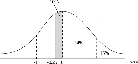
`ztext{-score (860)}\ = (x-mu)/sigma=(860-840)/80=0.25`
`ztext{-score (820)}\ =(820-840)/80=-0.25`
`ztext{-score (920)}\ =(920-840)/80=1`
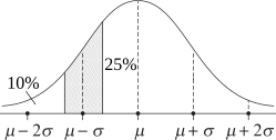
`text{50% of batteries have a life span below 840 hours (by definition)}`
`=>\ text{10% lie between 840 and 860 hours}`
`=>\ text{By symmetry, 10% lie between 820 and 840 hours}`
`=> P(-0.25<=z<=0)=10text{%}`
`:.\ text{Percentage between 820 and 920}`
`=P(-0.25<=z<=1)`
`=P(-0.25<=z<=0) + P(0<=z<=1)`
`=10+34`
`=44text{%}`
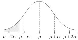
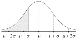
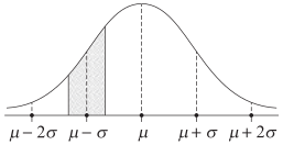
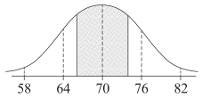
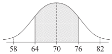
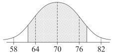
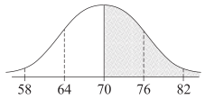
The scores on an examination are normally distributed with a mean of 70 and a standard deviation of 6. Michael received a score on the examination between the lower quartile and the upper quartile of the scores.
Which shaded region most accurately represents where Michael's score lies?
| A. | B. | ||
| C. | D. |
`A`
`text{68% of marks lie between 64 and 76 (mean ± 1 σ).}`
`text(50% of marks lie between)\ Q_1\ text(and)\ Q_3.`
`=> A`
A set of data is normally distributed with a mean of 48 and a standard deviation of 3.
Approximately what percentage of the scores lies between 39 and 45?
`A`
All the students in a class of 30 did a test.
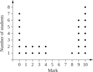
The marks, out of 10, are shown in the dot plot.
--- 1 WORK AREA LINES (style=lined) ---
Using the dot plot, calculate the percentage of the marks which lie within one standard deviation of the mean. (2 marks)
--- 4 WORK AREA LINES (style=lined) ---
--- 2 WORK AREA LINES (style=lined) ---
| i. | `text(Median)` | `= text(15th + 16th score)/2` |
| `= (4 + 8)/2` | ||
| `= 6` |
ii. `text(Lower limit) = 5.4 – 4.22 = 1.18`
`text(Upper limit) = 5.4 + 4.22 = 9.62`
`:.\ text(Percentage in between)`
`= 13/30 xx 100`
`= 43.33…`
`= 43text{% (nearest %)}`
iii. `text(The statement assumes the data is normally)`
`text(distributed which is not the case here.)`
The pulse rates of a large group of 18-year-old students are approximately normally distributed with a mean of 75 beats/minute and a standard deviation of 11 beats/minute.
The percentage of 18-year-old students with pulse rates less than 53 beats/minute or greater than 86 beats/minute is closest to
`D`
`mu=75,\ \ \ sigma=11`
`z text{-score (53)}=(x-mu) /sigma=(53-75)/11= -2`
`z text{-score (86)}= (86-75)/11=1`
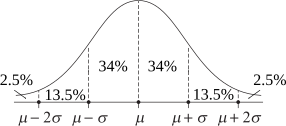
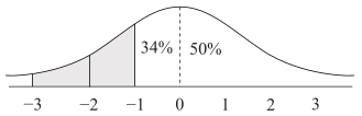
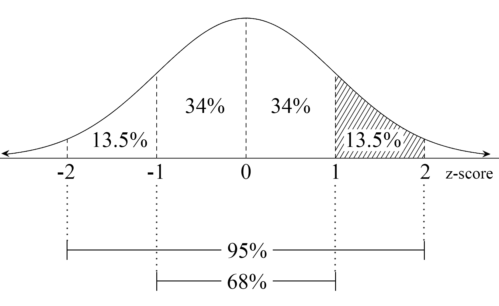
`text(From the diagram, the % of students that have a)`
`z text(-score below –2 or above 1)`
`=2.5+16=18.5 text(%)`
`=>D`
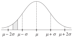
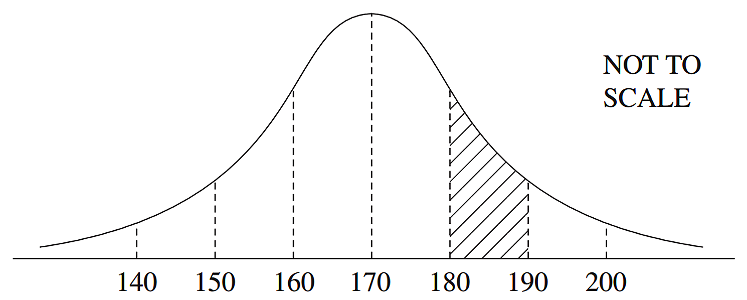
The normal distribution shown has a mean of 170 and a standard deviation of 10.
--- 1 WORK AREA LINES (style=lined) ---
--- 4 WORK AREA LINES (style=lined) ---
a. `1 <= text(z-score) <= 2`
b. `text(13.5%)`
a. `ztext{-score(180)}= (x-mu)/sigma= (180-170)/10= 1`
`ztext{-score(190)}= (190-170)/10= 2`
`:. 1 <= ztext(-score) <= 2`
| ii. | ![]() |
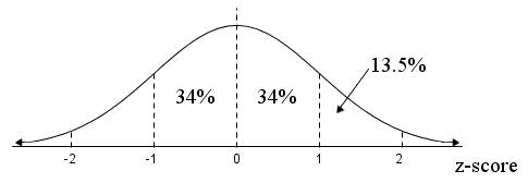
`text(From the graph above:)`
`text(13.5% lies in the shaded area.)`
In a normally distributed set of scores, the mean is 23 and the standard deviation is 5.
Approximately what percentage of the scores will lie between 18 and 33?
`D`
The weights of 10 000 newborn babies in NSW are normally distributed. These weights have a mean of 3.1 kg and a standard deviation of 0.35 kg.
How many of these newborn babies have a weight between 2.75 kg and 4.15 kg?
`D`
`text(Find)\ z text(-scores of 2.75 and 4.15 kg)`
| `z\ (2.75)` | `= (x – mu)/5 = (2.75 – 3.1)/0.35 = -1` |
| `z\ (4.15)` | `= (4.15 – 3.1)/0.35 = 3` |
`text(68% between)\ z=–1\ text(and 1)`
`=> text(34% between)\ z=–1\ text(and 0)`
`text(99.7% between)\ z=–3\ text(and 3)`
`=> text(49.85% between)\ z=0\ text(and)\ 3`
`:.%\ text(with)\ z text(-scores between)\ –1\ text(and 3)`
`= 34 + 49.85`
`=\ text(83.85%)`
`:.\ text(# Babies between 2.75 kg and 4.15 kg)`
`= text(83.85%) xx 10\ 000`
`= 8385`
`=> D`
In Broken Hill, the maximum temperature for each day has been recorded. The mean of these maximum temperatures during spring is 25.8°C, and their standard deviation is 4.2° C.
--- 1 WORK AREA LINES (style=lined) ---
You may assume that these maximum temperatures are normally distributed and that
• 68% of maximum temperatures have `z`-scores between –1 and 1
• 95% of maximum temperatures have `z`-scores between –2 and 2
• 99.7% of maximum temperatures have `z`-scores between –3 and 3. (3 marks)
--- 6 WORK AREA LINES (style=lined) ---
i. `mu = 25.8\ \ \ sigma = 4.2`
| `text(Using)\ \ \ \ z` | `= (x-mu)/sigma` |
| `-1` | `= (x-25.8)/4.2` |
| `x` `- 25.8` | `= -4.2` |
| `x` | `= 21.6°` |
`:.\ 21.6^@\ text(has a)\ z text(-score of) -1`
ii. `z text(-score of)\ 21.6 = -1`
`text(Find)\ z text(-score of 38.4)`
| `z\ (38.4)` | `= (38.4\ – 25.8)/4.2=3` |
`text(68% of scores are between)\ z= –1\ text(and 1)`
`=>\ text(34%)\ text(are between)\ z=–1\ text(and 0)`
`text(99.7% of scores are between)\ z= –3\ text(and 3)`
`=>\ text(49.85%)\ text(are between)\ z=0\ text(and 3)`
`:.\ text(% Temps between 21.6° and 38.4°)`
| `=\ text(34% + 49.85%)` |
| `=\ text(83.85%)` |
The marks in a class test are normally distributed. The mean is 100 and the standard deviation is 10.
--- 1 WORK AREA LINES (style=lined) ---
You may assume the following:
• 68% of marks have a `z`-score between –1 and 1
• 95% of marks have a `z`-score between –2 and 2
• 99.7% of marks have a `z`-score between –3 and 3. (2 marks)
--- 4 WORK AREA LINES (style=lined) ---
i. ` text(Given) \ \ mu=100,\ \ sigma=10`
`text(If mark is 115,`
| `ztext(-score)` | `=(115-mu)/sigma` |
| `=(115-100)/100` | |
| `=1.5` |
ii. `z text(-score = 0 when mark equals the mean)`
`:.\ text(Mary’s score was)\ 100`
| iii. `ztext(-score of)\ 110` | `=(110-100)/10=1` |
| `ztext(-score of)\ 80` | `=(80-100)/10=–2` |
`text(68% of marks lie between)\ z= –1 \ text(and)\ 1`
`=>text(34% lie between)\ z= 0\ text(and)\ 1`
`text(95% of marks lie between)\ z= –2 \ text(and)\ 2`
`=> text(47.5% lie between)\ z= –2\ text(and)\ 0`
`:.\ text(% marks between 80 and 110`
`=\ text(34% + 47.5%)`
`=\ text(81.5%)`
A machine produces nails. When the machine is set correctly, the lengths of the nails are normally distributed with a mean of 6.000 cm and a standard deviation of 0.040 cm.
To confirm the setting of the machine, three nails are randomly selected. In one sample the lengths are 5.950, 5.983 and 6.140.
The setting of the machine needs to be checked when the lengths of two or more nails in a sample lie more than 1 standard deviation from the mean.
Does the setting on the machine need to be checked? Justify your answer with suitable calculations. (2 marks)
--- 4 WORK AREA LINES (style=lined) ---
`text(Settings need to be checked.)`
`mu = 6.000,\ \ sigma = 0.040`
`text(Limits for ±1 σ:)`
`6.000 + 0.040 = 6.040\ text{(upper)}`
`6.000-0.040 = 5.960\ text{(lower)}`
| `text(Chosen nails:)\ \ 5.950` | `=>\ text(outside limits)` |
| `5.983` | `=>\ text(inside)` |
| `6.140` | `=>\ text(outside)` |
`text(S)text(ince 2 nails are outside 1 σ limits)`
`:.\ text(Settings need to be checked.)`
There are 60 000 students sitting a state-wide examination. If the results form a normal distribution, how many students would be expected to score a result between 1 and 2 standard deviations above the mean?
You may assume for normally distributed data that:
`A`
`text(S)text(ince 68% between)\ z=1\ text(and)\ -1`
` => text(34% between)\ z=0\ text(and)\ 1`
`text(Likewise, 95% between)\ z=2\ text(and) -2`
` => text(47.5% between)\ z=0\ text(and)\ 2`
`:.\ text(% between)\ z=1\ text(and)\ 2`
`=47.5-34`
`=13.5 text(%)`
`:.\ text(Students between)\ \ z=1\ text(and)\ \ z=2`
`=13.5 text(%)xx60\ 000`
`=8100`
`=>\ A`