2adv-std2-common

Statistics, STD2 S4 2025 HSC 25

In a research study, participants were asked to record the number of minutes they spent watching television and the number of minutes they spent exercising each day over a period of 3 months. The averages for each participant were recorded and graphed.

Describe the bivariate dataset in terms of its form and direction. (2 marks)
Form: ..................................................................
Direction: ............................................................
--- 0 WORK AREA LINES (style=lined) ---

The equation of the least-squares regression line for this dataset is

$y=64.3-0.7 x$

Interpret the values of the slope and $y$-intercept of the regression line in the context of this dataset. (2 marks)

--- 6 WORK AREA LINES (style=lined) ---
Jo spends an average of 42 minutes per day watching television.
Use the equation of the regression line to determine how many minutes on average Jo is expected to exercise each day. (1 mark)

--- 4 WORK AREA LINES (style=lined) ---
Explain why it is NOT appropriate to extrapolate the regression line to predict the average number of minutes of exercise per day for someone who watches an average of 2 hours of television per day. (1 mark)

--- 4 WORK AREA LINES (style=lined) ---

Show Answers Only

a. $\text{Form: Linear. Direction: Negative}$

Show Worked Solution

a. $\text{Form: Linear}$

$\text{Direction: Negative}$

b. $\text{Slope}=-0.7$

$\text{This means that for each added minute of watching television per day, a participant, on average,}$

$\text{will exercise for 0.7 minutes less.}$

$y \text{-intercept}=64.3$

$\text{If someone watches no television, the LSRL predicts they will exercise for 64.3 minutes per day.}$

c. $\text{At} \ \ x=42:$

$y=64.3-0.7 \times 42=34.9$

$\therefore \ \text{Jo is expected to exercise for 34.9 minutes}$

d. $\text{At} \ \ x=120\ \text{(2 hours),} \ \ y=64.3-0.7 \times 120=-19.7$

$\text{The model predicts a negative value for time spent exercising, which is not possible.}$

Algebra, STD2 A4 2025 HSC 2 MC

Which graph could represent $y=4^x$ ?

Show Answers Only

$A$

Show Worked Solution

$\Rightarrow A$

Functions, 2ADV F2 2025 HSC 2 MC

Which graph could represent $y=4^x$ ?

Show Answers Only

$A$

Show Worked Solution

$\Rightarrow A$

Statistics, STD2 S5 2025 HSC 40

In a flock of 12 600 sheep, the ratio of males to females is $1:20$.
The weights of the male sheep are normally distributed with a mean of 76.2 kg and a standard deviation of 6.8 kg.
In the flock, 15 of the male sheep each weigh more than $x$ kg.
Find the value of $x$. (4 marks)

--- 10 WORK AREA LINES (style=lined) ---
The weights of the female sheep are also normally distributed but have a smaller mean and smaller standard deviation than the weights of male sheeр.
Explain whether it could be expected that 300 of the females from the flock each weigh more than $x$ kg, where $x$ is the value found in part (a). (1 mark)

--- 6 WORK AREA LINES (style=lined) ---

Show Answers Only

a. $x=89.8 \ \text{kg}$

b. $\text{Female sheep} \ \%=\dfrac{300}{12\,000}=0.025 \%\ (z \text{-score = 2)}$

$\text{Given} \ \ \bar{x}_f<\bar{x}_m \ \ \text{and} \ \ s_f<s_m$

$\text{Consider the value of}\ x_f\ \text{when \(z$-score = 2}:\)

$\Rightarrow x_f=\bar{x}_f+2 \times s_f \leq x_m$

$\therefore \ \text{It is not expected that 300 females weigh > 89.8 kg.}$

Show Worked Solution

a. $12\,600 \ \text{sheep} \ \Rightarrow \ \text{male : female}=1:20$

$\text{Number of sheep in “1 part”} = \dfrac{12\,600}{21}=600$

$\Rightarrow \ \text{male : female}=600:12\,000$

$\text{male sheep} \ \%=\dfrac{15}{600}=0.025\%$

$z \text{-score }(0.025 \%)=2$

$\text{Using } \ z=\dfrac{x-\bar{x}}{s}, \ \text{find} \ \ x_m:$

$2$	$=\dfrac{x_m-76.2}{6.8}$
$x_m$	$=76.2+2 \times 6.8=89.8 \ \text{kg}$

b. $\text{Female sheep} \ \%=\dfrac{300}{12\,000}=0.025 \%\ (z \text{-score = 2)}$

$\text{Given} \ \ \bar{x}_f<\bar{x}_m \ \ \text{and} \ \ s_f<s_m$

$\text{Consider the value of}\ x_f\ \text{when \(z$-score = 2}:\)

$\Rightarrow x_f=\bar{x}_f+2 \times s_f \leq x_m$

$\therefore \ \text{It is not expected that 300 females weigh > 89.8 kg.}$

Statistics, 2ADV S3 2025 HSC 23

In a flock of 12 600 sheep, the ratio of males to females is $1:20$.
The weights of the male sheep are normally distributed with a mean of 76.2 kg and a standard deviation of 6.8 kg.
In the flock, 15 of the male sheep each weigh more than $x$ kg.
Find the value of $x$. (4 marks)

--- 10 WORK AREA LINES (style=lined) ---
The weights of the female sheep are also normally distributed but have a smaller mean and smaller standard deviation than the weights of male sheeр.
Explain whether it could be expected that 300 of the females from the flock each weigh more than $x$ kg, where $x$ is the value found in part (a). (1 mark)

--- 6 WORK AREA LINES (style=lined) ---

Show Answers Only

a. $x=89.8 \ \text{kg}$

b. $\text{Female sheep} \ \%=\dfrac{300}{12\,000}=0.025 \%\ (z \text{-score = 2)}$

$\text{Given} \ \ \bar{x}_f<\bar{x}_m \ \ \text{and} \ \ s_f<s_m$

$\text{Consider the value of}\ x_f\ \text{when \(z$-score = 2}:\)

$\Rightarrow x_f=\bar{x}_f+2 \times s_f \leq x_m$

$\therefore \ \text{It is not expected that 300 females weigh > 89.8 kg.}$

Show Worked Solution

a. $12\,600 \ \text{sheep} \ \Rightarrow \ \text{male : female}=1:20$

$\text{Number of sheet in “1 part”} = \dfrac{12\,600}{21}=600$

$\Rightarrow \ \text{male : female}=600:12\,000$

$\text{male sheep} \ \%=\dfrac{15}{600}=0.025\%$

$z \text{-score }(0.025 \%)=2$

$\text{Using } \ z=\dfrac{x-\bar{x}}{s}, \ \text{find} \ \ x_m:$

$2$	$=\dfrac{x_m-76.2}{6.8}$
$x_m$	$=76.2+2 \times 6.8=89.8 \ \text{kg}$

b. $\text{Female sheep} \ \%=\dfrac{300}{12\,000}=0.025 \%\ (z \text{-score = 2)}$

$\text{Given} \ \ \bar{x}_f<\bar{x}_m \ \ \text{and} \ \ s_f<s_m$

$\text{Consider the value of}\ x_f\ \text{when \(z$-score = 2}:\)

$\Rightarrow x_f=\bar{x}_f+2 \times s_f \leq x_m$

$\therefore \ \text{It is not expected that 300 females weigh > 89.8 kg.}$

Statistics, STD2 S4 2025 25

Describe the bivariate dataset in terms of its form and direction. (2 marks)
Form: ..................................................................
Direction: ............................................................
--- 0 WORK AREA LINES (style=lined) ---

The equation of the least-squares regression line for this dataset is

$y=64.3-0.7 x$

Interpret the values of the slope and $y$-intercept of the regression line in the context of this dataset. (2 marks)

--- 6 WORK AREA LINES (style=lined) ---
Jo spends an average of 42 minutes per day watching television.
Use the equation of the regression line to determine how many minutes on average Jo is expected to exercise each day. (1 mark)

--- 4 WORK AREA LINES (style=lined) ---
Explain why it is NOT appropriate to extrapolate the regression line to predict the average number of minutes of exercise per day for someone who watches an average of 2 hours of television per day. (1 mark)

--- 4 WORK AREA LINES (style=lined) ---

Show Answers Only

a. $\text{Form: Linear. Direction: Negative}$

Show Worked Solution

a. $\text{Form: Linear}$

$\text{Direction: Negative}$

b. $\text{Slope}=-0.7$

$\text{This means that for each added minute of watching television per day, a participant, on average,}$

$\text{will exercise for 0.7 minutes less.}$

$y \text{-intercept}=64.3$

$\text{If someone watches no television, the LSRL predicts they will exercise for 64.3 minutes per day.}$

c. $\text{At} \ \ x=42:$

$y=64.3-0.7 \times 42=34.9$

$\therefore \ \text{Jo is expected to exercise for 34.9 minutes}$

d. $\text{At} \ \ x=120\text{(2 hours),} \ \ y=64.3-0.7 \times 120=-19.7$

$\text{The model predicts a negative value for time spent exercising, which is not possible.}$

Statistics, 2ADV S2 2025 HSC 14

Describe the bivariate dataset in terms of its form and direction. (2 marks)
Form: ..................................................................
Direction: ............................................................
--- 0 WORK AREA LINES (style=lined) ---

The equation of the least-squares regression line for this dataset is

$y=64.3-0.7 x$

Interpret the values of the slope and $y$-intercept of the regression line in the context of this dataset. (2 marks)

--- 6 WORK AREA LINES (style=lined) ---
Jo spends an average of 42 minutes per day watching television.
Use the equation of the regression line to determine how many minutes on average Jo is expected to exercise each day. (1 mark)

--- 4 WORK AREA LINES (style=lined) ---
Explain why it is NOT appropriate to extrapolate the regression line to predict the average number of minutes of exercise per day for someone who watches an average of 2 hours of television per day. (1 mark)

--- 4 WORK AREA LINES (style=lined) ---

Show Answers Only

a. $\text{Form: Linear}$

$\text{Direction: Negative}$

b. $\text{Slope}=-0.7$

$\text{This means that for each added minute of watching television per day, a participant, on average,}$

$\text{will exercise for 0.7 minutes less.}$

$y \text{-intercept}=64.3$

$\text{If someone watches no television, the LSRL predicts they will exercise for 64.3 minutes per day.}$

c. $\text{34.9 minutes}$

d. $\text{At} \ \ x=120\ \text{(2 hours),} \ \ y=64.3-0.7 \times 120=-19.7$

$\text{The model predicts a negative value for time spent exercising, which is not possible.}$

Show Worked Solution

a. $\text{Form: Linear}$

$\text{Direction: Negative}$

b. $\text{Slope}=-0.7$

$\text{This means that for each added minute of watching television per day, a participant, on average,}$

$\text{will exercise for 0.7 minutes less.}$

$y \text{-intercept}=64.3$

$\text{If someone watches no television, the LSRL predicts they will exercise for 64.3 minutes per day.}$

c. $\text{At} \ \ x=42:$

$y=64.3-0.7 \times 42=34.9$

$\therefore \ \text{Jo is expected to exercise for 34.9 minutes}$

d. $\text{At} \ \ x=120\ \text{(2 hours),} \ \ y=64.3-0.7 \times 120=-19.7$

$\text{The model predicts a negative value for time spent exercising, which is not possible.}$

Algebra, STD2 A4 2025 HSC 20

The graph of a quadratic function represented by the equation $h=t^2-8 t+12$ is shown.

Find the values of $t$ and $h$ at the turning point of the graph. (2 marks)

--- 6 WORK AREA LINES (style=lined) ---
The graph shows $h=12$ when $t=0$.
What is the other value of $t$ for which $h=12$? (1 mark)

--- 3 WORK AREA LINES (style=lined) ---

Show Answers Only

a. $\text{Turning point at} \ \ (4,-4)$

b. $t=8$

Show Worked Solution

a. $\text{Axis of quadratic occurs when}\ \ t= \dfrac{2+6}{2} = 4$

$\text{At} \ \ t=4:$

$h=4^2-8 \times 4+12=-4$

$\therefore \ \text{Turning point at} \ \ (4,-4)$

b. $\text {When} \ \ h=12:$

$t^2-8 t+12$	$=12$
$t(t-8)$	$=0$

$\therefore \ \text{Other value:} \ \ t=8$

Functions, 2ADV F1 2025 HSC 11

The graph of a quadratic function represented by the equation $h=t^2-8 t+12$ is shown.

Find the values of $t$ and $h$ at the turning point of the graph. (2 marks)

--- 6 WORK AREA LINES (style=lined) ---
The graph shows $h=12$ when $t=0$.
What is the other value of $t$ for which $h=12$? (1 mark)

--- 3 WORK AREA LINES (style=lined) ---

Show Answers Only

a. $\text{Turning point at} \ \ (4,-4)$

b. $t=8$

Show Worked Solution

a. $\text{Strategy 1 (no calculus)}$

$\text{Axis of quadratic occurs when}\ \ t= \dfrac{2+6}{2} = 4$

$\text{At} \ \ t=4:$

$h=4^2-8 \times 4+12=-4$

$\therefore \ \text{Turning point at} \ \ (4,-4)$

$\text{Strategy 2 (using calculus)}$

$h=t^2-8 t+12$

$h^{\prime}=2 t-8$

$\text{Find \(t$ when} \ \ h^{\prime}=0:\)

$2 t-8=0 \ \Rightarrow \ t=4$

b. $\text {When} \ \ h=12:$

$t^2-8 t+12$	$=12$
$t(t-8)$	$=0$

$\therefore \ \text{Other value:} \ \ t=8$

Probability, STD2 S2 2025 HSC 13 MC

A ten-sided die has faces numbered 1 to 10 .

The die is constructed so that the probability of obtaining the number 1 is greater than the probability of obtaining any of the other numbers. The numbers 2 to 10 are equally likely to occur.

When the die is rolled 153 times, a 1 is obtained 72 times.

By using the relative frequency of rolling a 1, which of the following is the best estimate for the probability of rolling a 10 ?

$\dfrac{1}{17}$
$\dfrac{1}{11}$
$\dfrac{1}{10}$
$\dfrac{1}{9}$

Show Answers Only

$A$

Show Worked Solution

$P(1) = \dfrac{72}{153}=\dfrac{8}{17} $

$\text{Let}\ \ p=P(2)=P(3) = … =P(10) $

$\dfrac{8}{17}+9p$	$=1$
$9p$	$=1-\dfrac{8}{17}$
$p$	$=\dfrac{1}{17}$

$\Rightarrow A$

Probability, 2ADV S1 2025 HSC 7 MC

A ten-sided die has faces numbered 1 to 10 .

The die is constructed so that the probability of obtaining the number 1 is greater than the probability of obtaining any of the other numbers. The numbers 2 to 10 are equally likely to occur.

When the die is rolled 153 times, a 1 is obtained 72 times.

By using the relative frequency of rolling a 1, which of the following is the best estimate for the probability of rolling a 10 ?

$\dfrac{1}{17}$
$\dfrac{1}{11}$
$\dfrac{1}{10}$
$\dfrac{1}{9}$

Show Answers Only

$A$

Show Worked Solution

$P(1) = \dfrac{72}{153}=\dfrac{8}{17} $

$\text{Let}\ \ p=P(2)=P(3) = … =P(10) $

$\dfrac{8}{17}+9p$	$=1$
$9p$	$=1-\dfrac{8}{17}$
$p$	$=\dfrac{1}{17}$

$\Rightarrow A$

v1 Algebra, STD2 A4 2021 HSC 10 MC

Which of the following best represents the graph of $y = 5 (0.4)^{x}$ ?

Show Answers Only

$D$

Show Worked Solution

$\text{By elimination:}$

♦ Mean mark 41%.

$\text{When}\ x = 0, \ y = 5 \times (0.4)^0 = 5$

$\rightarrow\ \text{Eliminate B and C} $

$\text{As}\ \ x \rightarrow \infty, \ y \rightarrow 0 $

$\rightarrow\ \text{Eliminate A} $

$\Rightarrow D$

v1 Algebra, STD2 A4 2022 HSC 24

A chef believes that the time it takes to defrost a turkey (`D` hours) varies inversely with the room temperature (`T^\circ \text{C}`). The chef observes that at a room temperature of `20^\circ \text{C}`, it takes 15 hours for the turkey to fully defrost.

Find the equation relating `D` and `T`. (2 marks)

--- 4 WORK AREA LINES (style=lined) ---
By first completing this table of values, graph the relationship between temperature and time. (2 marks)

\begin{array} {|l|c|c|c|c|c|}
\hline
\rule{0pt}{2.5ex} \ \ T\ \ \rule[-1ex]{0pt}{0pt} & \ \ \ 10\ \ \ & \ \ 15\ \ \ & \ \ \ 20\ \ \ & \ \ \ 25\ \ \ & \ \ \ 30\ \ \ \\
\hline
\rule{0pt}{2.5ex} \ \ D\ \ \rule[-1ex]{0pt}{0pt} & \ \ \ \ & \ \ \ & \ \ \ \ & \ \ \ \ & \ \ \ \\
\hline
\end{array}

--- 0 WORK AREA LINES (style=lined) ---

Show Answers Only

a. `D \prop 1/T\ \ =>\ \ D=k/T`

	`15`	`=k/20`
	`k`	`=15 xx 20=300`

`:.D=300/T`

\begin{array} {|l|c|c|c|c|c|}
\hline
\rule{0pt}{2.5ex} \ \ T\ \ \rule[-1ex]{0pt}{0pt} & \ \ \ 10\ \ \ & \ \ 15\ \ \ & \ \ \ 20\ \ \ & \ \ \ 25\ \ \ & \ \ \ 30\ \ \ \\
\hline
\rule{0pt}{2.5ex} \ \ D\ \ \rule[-1ex]{0pt}{0pt} & \ \ \ 30\ \ \ & \ \ 20\ \ \ & \ \ \ 15\ \ \ & \ \ \ 12\ \ \ & \ \ \ 10\ \ \ \\
\hline
\end{array}

Show Worked Solution

a. `D \prop 1/T\ \ =>\ \ D=k/T`

	`15`	`=k/20`
	`k`	`=15 xx 20=300`

`:.D=300/T`

\begin{array} {|l|c|c|c|c|c|}
\hline
\rule{0pt}{2.5ex} \ \ D\ \ \rule[-1ex]{0pt}{0pt} & \ \ \ 10\ \ \ & \ \ 15\ \ \ & \ \ \ 20\ \ \ & \ \ \ 25\ \ \ & \ \ \ 30\ \ \ \\
\hline
\rule{0pt}{2.5ex} \ \ T\ \ \rule[-1ex]{0pt}{0pt} & 30 & 20 & 15 & 12 & 10 \\
\hline
\end{array}

Statistics, 2ADV S2 2024 HSC 16

Flowers were planted in two gardens (Garden A and Garden B).

On a particular day, 25 flowers were randomly selected from each garden and their heights measured in millimetres.

The data are represented in parallel box-plots.

Compare the two datasets by examining the skewness of the distributions, and the measures of central tendency and spread. (3 marks)

--- 8 WORK AREA LINES (style=lined) ---

Show Answers Only

$\text{Skewness comparison:}$

$\rightarrow\ \text{Garden A is negatively skewed while Garden B is positively skewed.}$

$\text{Measures of central tendency comparison:}$

$\rightarrow\ \text{IQR (A)}\ \approx 17\ \text{ is greater than IQR (B)}\ \approx 9$

$\rightarrow\ \text{This means the middle 50% of data points of B are more closely clustered} $
$\text{around the median than A.}$

$\text{Spread comparison:}$

$\rightarrow\ \text{Range (A)}\ \approx 39\ \text{is less than range (B)}\ \approx 28$

$\rightarrow\ \text{This means the spread of data points of A is wider than the spread of data points of B.}$

$\text{Overall, flowers from Garden B will tend to be higher than Garden A flowers as well as exhibiting}$
$\text{a larger range of heights.}$

Show Worked Solution

$\text{Skewness comparison:}$

$\rightarrow\ \text{Garden A is negatively skewed while Garden B is positively skewed.}$

$\text{Measures of central tendency comparison:}$

$\rightarrow\ \text{IQR (A)}\ \approx 17\ \text{ is greater than IQR (B)}\ \approx 9$

$\rightarrow\ \text{This means the middle 50% of data points of B are more closely clustered}$
$\text{around the median than A.}$

$\text{Spread comparison:}$

$\rightarrow\ \text{Range (A)}\ \approx 39\ \text{is less than range (B)}\ \approx 28$

$\rightarrow\ \text{This means the spread of data points of A is wider than the spread of data points of B.}$

$\text{Overall, flowers from Garden B will tend to be higher than Garden A flowers as well as exhibiting}$
$\text{a larger range of heights.}$

L&E, 2ADV E1 2024 HSC 13

The graph shows the populations of two different animals, $W$ and $K$, in a conservation park over time. The $y$-axis is the size of the population and the $x$-axis is the number of years since 1985 .

Population $W$ is modelled by the equation $y=A \times(1.055)^x$.

Population $K$ is modelled by the equation $y=B \times(0.97)^x$.

Complete the table using the information provided. (3 marks)

\begin{array}{|l|c|c|}
\hline
\rule{0pt}{2.5ex}\rule[-1ex]{0pt}{0pt}&\text {Population } W & \text {Population } K \\
\hline
\rule{0pt}{2.5ex}\text { Population in 1985 }\rule[-1ex]{0pt}{0pt} & A=34 & B=\ \ \ \ \ \\
\hline
\rule{0pt}{2.5ex}\text { Percentage yearly change in the population }\rule[-1ex]{0pt}{0pt} & & \\
\hline
\rule{0pt}{2.5ex}\text { Predicted population when } x=50 \rule[-1ex]{0pt}{0pt}& & 61 \\
\hline
\end{array}

--- 5 WORK AREA LINES (style=lined) ---

Show Answers Only

\begin{array}{|l|c|c|}
\hline
\rule{0pt}{2.5ex}\rule[-1ex]{0pt}{0pt}&\text {Population } W & \text {Population } K \\
\hline
\rule{0pt}{2.5ex}\text { Population in 1985 }\rule[-1ex]{0pt}{0pt} & A=34 & B=280 \\
\hline
\rule{0pt}{2.5ex}\text { Percentage yearly change in the population }\rule[-1ex]{0pt}{0pt} &+5.5\% & -3.0\%\\
\hline
\rule{0pt}{2.5ex}\text { Predicted population when } x=50 \rule[-1ex]{0pt}{0pt}&494 & 61 \\
\hline
\end{array}

Show Worked Solution

\begin{array}{|l|c|c|}
\hline
\rule{0pt}{2.5ex}\rule[-1ex]{0pt}{0pt}&\text {Population } W & \text {Population } K \\
\hline
\rule{0pt}{2.5ex}\text { Population in 1985 }\rule[-1ex]{0pt}{0pt} & A=34 & B=280 \\
\hline
\rule{0pt}{2.5ex}\text { Percentage yearly change in the population }\rule[-1ex]{0pt}{0pt} &+5.5\% & -3.0\%\\
\hline
\rule{0pt}{2.5ex}\text { Predicted population when } x=50 \rule[-1ex]{0pt}{0pt}&494 & 61 \\
\hline
\end{array}

$\text{Calculations:}$

$\text{Population } W: \ (1.055)^x \Rightarrow \text { increase of 5.5% each year}$

$\text {Population } K: \ (0.97)^x \Rightarrow 1-0.97=0.03 \Rightarrow \text { decrease of 3.0% each year}$

$\text {Predicted population }(W)=34 \times(1.055)^{50}=494$

Algebra, STD2 A4 2024 HSC 22

Population $W$ is modelled by the equation $y=A \times(1.055)^x$.

Population $K$ is modelled by the equation $y=B \times(0.97)^x$.

Complete the table using the information provided. (3 marks)

--- 5 WORK AREA LINES (style=lined) ---

Show Answers Only

\begin{array}{|l|c|c|}
\hline
\rule{0pt}{2.5ex}\rule[-1ex]{0pt}{0pt}&\text {Population } W & \text {Population } K \\
\hline
\rule{0pt}{2.5ex}\text { Population in 1985 }\rule[-1ex]{0pt}{0pt} & A=34 & B=280 \\
\hline
\rule{0pt}{2.5ex}\text { Percentage yearly change in the population }\rule[-1ex]{0pt}{0pt} &+5.5\% & -3.0\%\\
\hline
\rule{0pt}{2.5ex}\text { Predicted population when } x=50 \rule[-1ex]{0pt}{0pt}&494 & 61 \\
\hline
\end{array}

Show Worked Solution

\begin{array}{|l|c|c|}
\hline
\rule{0pt}{2.5ex}\rule[-1ex]{0pt}{0pt}&\text {Population } W & \text {Population } K \\
\hline
\rule{0pt}{2.5ex}\text { Population in 1985 }\rule[-1ex]{0pt}{0pt} & A=34 & B=280 \\
\hline
\rule{0pt}{2.5ex}\text { Percentage yearly change in the population }\rule[-1ex]{0pt}{0pt} &+5.5\% & -3.0\%\\
\hline
\rule{0pt}{2.5ex}\text { Predicted population when } x=50 \rule[-1ex]{0pt}{0pt}&494 & 61 \\
\hline
\end{array}

$\text{Calculations:}$

$\text{Population } W: \ (1.055)^x \Rightarrow \text { increase of 5.5% each year}$

$\text {Population } K: \ (0.97)^x \Rightarrow 1-0.97=0.03 \Rightarrow \text { decrease of 3.0% each year}$

$\text {Predicted population }(W)=34 \times(1.055)^{50}=494$

Mean mark 51%.

Financial Maths, 2ADV M1 2024 HSC 26

Twenty-five years ago, Phoenix deposited a single sum of money into a new bank account, earning 2.4% interest per annum compounding monthly.

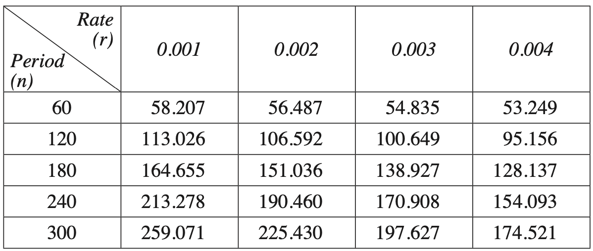
Present value interest factors for an annuity of $1 for various interest rates $(r)$ and numbers of periods $(n)$ are given in the table.

Phoenix made the following withdrawals from this account.

$2000 at the end of each month for the first 15 years, starting at the end of the first month.
$1200 at the end of each month for the next 10 years, starting at the end of the 181st month after the account was opened.

Calculate the minimum sum that Phoenix could have deposited in order to make these withdrawals. (4 marks)

--- 10 WORK AREA LINES (style=lined) ---

Show Answers Only

$\text{Minimum deposit}\ = $391\,344.80$

Show Worked Solution

$\text{1st Annuity}$

$\text{Find PVA for \$2000 paid monthly for 1st 15 years:}$

$r= \dfrac{2.4%}{12} = 0.2\% = 0.002$

$\text{Total payments (to Phoenix)}\ = 15 \times 12 = 180$

$\text{PVA factor (from table)}\ = 151.036$

$\text{PVA (1st annuity)}\ = 2000 \times 151.036 = $302\,072$

♦ Mean mark 51%.

$\text{2nd Annuity}$

$\text{Find PVA for \$1200 paid monthly from year 16 to 25:}$

$\text{PVA (2nd annuity) = PVA (25 years) }-\text{ PVA (15 years)}$

$r= \dfrac{2.4%}{12} = 0.2\% = 0.002$

$\text{Total payments (25 years)}\ = 25 \times 12 = 300$

$\text{PVA factors (from table): 225.430 (25 years), 151.036 (15 years)}$

$\text{PVA (2nd annuity)}$	$=(1200 \times 225.430)-(1200 \times 151.036)$
	$=$89\,272.80$

$\therefore\ \text{Minimum deposit}\ = 302\,072+89\,272.80 = $391\,344.80$

Financial Maths, STD2 F5 2024 HSC 41

Twenty-five years ago, Phoenix deposited a single sum of money into a new bank account, earning 2.4% interest per annum compounding monthly.

Present value interest factors for an annuity of $1 for various interest rates $(r)$ and numbers of periods $(n)$ are given in the table.

Phoenix made the following withdrawals from this account.

$2000 at the end of each month for the first 15 years, starting at the end of the first month.
$1200 at the end of each month for the next 10 years, starting at the end of the 181st month after the account was opened.

Calculate the minimum sum that Phoenix could have deposited in order to make these withdrawals. (4 marks)

--- 10 WORK AREA LINES (style=lined) ---

Show Answers Only

$\text{Minimum deposit}\ = $391\,344.80$

Show Worked Solution

$\text{1st Annuity}$

$\text{Find PVA for \$2000 paid monthly for 1st 15 years:}$

$r= \dfrac{2.4%}{12} = 0.2\% = 0.002$

$\text{Total payments (to Phoenix)}\ = 15 \times 12 = 180$

$\text{PVA factor (from table)}\ = 151.036$

$\text{PVA (1st annuity)}\ = 2000 \times 151.036 = $302\,072$

♦♦ Mean mark 39%.

$\text{2nd Annuity}$

$\text{Find PVA for \$1200 paid monthly from year 16 to 25:}$

$\text{PVA (2nd annuity) = PVA (25 years) }-\text{ PVA (15 years)}$

$r= \dfrac{2.4%}{12} = 0.2\% = 0.002$

$\text{Total payments (25 years)}\ = 25 \times 12 = 300$

$\text{PVA factors (from table): 225.430 (25 years), 151.036 (15 years)}$

$\text{PVA (2nd annuity)}$	$=(1200 \times 225.430)-(1200 \times 151.036)$
	$=$89\,272.80$

$\therefore\ \text{Minimum deposit}\ = 302\,072+89\,272.80 = $391\,344.80$

Statistics, 2ADV S2 2024 HSC 21

A researcher is studying anacondas (a type of snake).

A dataset recording the age (in years) and length (in cm) of female and male anacondas is displayed on the graph.

Anacondas reach maturity at about 4 years of age.

Write THREE observations about anacondas that may be made from the scatterplot. (Note: No calculations are required.) (3 marks)

--- 6 WORK AREA LINES (style=lined) ---

Show Answers Only

$\text{Answers could include any three of the following:}$

$→\ \text{Female anacondas are longer than males of the equivalent age.}$

$→\ \text{Female anacondas grow more quickly than male anacondas from birth until}$

$\text{maturity which can be seen by the steeper gradient of the LOBF for each dataset}$

$\text{over this period.}$

$→\ \text{Female anacondas continue to grow to at least 10 years of age, well past their}$

$\text{age of maturity at 4 years of age.}$

$→\ \text{Male anacondas’ growth slows noticeably and flattens out once they hit their}$

$\text{age of maturity at 4 years old.}$

Show Worked Solution

$\text{Answers could include any three of the following:}$

$→\ \text{Female anacondas are longer than males of the equivalent age.}$

$→\ \text{Female anacondas grow more quickly than male anacondas from birth until}$

$\text{maturity which can be seen by the steeper gradient of the LOBF for each dataset}$

$\text{over this period.}$

$→\ \text{Female anacondas continue to grow to at least 10 years of age, well past their}$

$\text{age of maturity at 4 years of age.}$

$→\ \text{Male anacondas’ growth slows noticeably and flattens out once they hit their}$

$\text{age of maturity at 4 years old.}$

Statistics, 2ADV S3 2024 HSC 23

A random variable is normally distributed with mean 0 and standard deviation 1. The table gives the probability that this random variable is less than $z$.

\begin{array} {|c|c|c|c|c|c|c|c|c|c|}
\hline
\rule{0pt}{2.5ex} z \rule[-1ex]{0pt}{0pt} & 0.6 & 0.7 & 0.8 & 0.9 & 1.0 & 1.1 & 1.2 & 1.3 & 1.4 \\
\hline
\rule{0pt}{2.5ex} \textit{Probability} \rule[-1ex]{0pt}{0pt} & 0.7257 & 0.7580 & 0.7881 & 0.8159 & 0.8413 & 0.8643 & 0.8849 & 0.9032 & 0.9192 \\
\hline
\end{array}

The probability values given in the table for different values of $z$ are represented by the shaded area in the following diagram.

The scores in a university examination with a large number of candidates are normally distributed with mean 58 and standard deviation 15.

By calculating a $z$-score, find the percentage of scores that are between 58 and 70. (2 marks)
--- 4 WORK AREA LINES (style=lined) ---
Explain why the percentage of scores between 46 and 70 is twice your answer to part (a). (1 mark)
--- 2 WORK AREA LINES (style=lined) ---
By using the values in the table above, find an approximate minimum score that a candidate would need to be placed in the top 10% of the candidates. (2 marks)
--- 4 WORK AREA LINES (style=lined) ---

Show Answers Only

a. $28.81%$

b. $\text{Normal distribution is symmetrical about the mean (58).}$

$\text{Since 70 and 46 are both the same distance (12) from the mean, the percentage}$

$\text{of scores in this range will be twice the answer in part (a).}$

c. $\text{Approx minimum score = 78%}$

Show Worked Solution

a. $z\text{-score (58)}\ =\dfrac{x-\mu}{\sigma} = \dfrac{58-58}{15}=0$

$z\text{-score (70)}\ = \dfrac{70-58}{15}=0.8$

$\text{Using table:}$

$\text{% between 58–70}\ =0.7881-0.5=0.2881=28.81%$

b. $\text{Normal distribution is symmetrical about the mean (58).}$

$\text{Since 70 and 46 are both the same distance (12) from the mean, the percentage}$

$\text{of scores in this range will be twice the answer in part (a).}$

c. $z\text{-score 1.3 has a table value 0.9032}$

$1-0.9032=0.0968\ \Rightarrow\ \text{i.e. 9.68% of students score higher.}$

$\text{Find}\ x\ \text{for a}\ z\text{-score of 1.3:}$

$1.3$	$=\dfrac{x-58}{15}$
$x$	$=1.3 \times 15 +58$
	$=77.5$

$\therefore\ \text{Approx minimum score = 78%}$

Statistics, STD2 S5 2024 HSC 35

A random variable is normally distributed with mean 0 and standard deviation 1. The table gives the probability that this random variable is less than $z$.

The probability values given in the table for different values of $z$ are represented by the shaded area in the following diagram.

The scores in a university examination with a large number of candidates are normally distributed with mean 58 and standard deviation 15.

By calculating a $z$-score, find the percentage of scores that are between 58 and 70. (2 marks)
--- 4 WORK AREA LINES (style=lined) ---
Explain why the percentage of scores between 46 and 70 is twice your answer to part (a). (1 mark)
--- 2 WORK AREA LINES (style=lined) ---
By using the values in the table above, find an approximate minimum score that a candidate would need to be placed in the top 10% of the candidates. (2 marks)
--- 4 WORK AREA LINES (style=lined) ---

Show Answers Only

a. $28.81%$

b. $\text{Normal distribution is symmetrical about the mean (58).}$

$\text{Since 70 and 46 are both the same distance (12) from the mean, the}$

$\text{percentage of scores in this range will be twice the answer in part (a).}$

c. $\text{Approx minimum score = 78%}$

Show Worked Solution

a. $z\text{-score (58)}\ =\dfrac{x-\mu}{\sigma} = \dfrac{58-58}{15}=0$

$z\text{-score (70)}\ = \dfrac{70-58}{15}=0.8$

$\text{Using table:}$

$\text{% between 58–70}\ =0.7881-0.5=0.2881=28.81%$

♦♦ Mean mark (a) 36%.

b. $\text{Normal distribution is symmetrical about the mean (58).}$

$\text{Since 70 and 46 are both the same distance (12) from the mean, the}$

$\text{percentage of scores in this range will be twice the answer in part (a).}$

♦♦♦ Mean mark (b) 19%.

c. $z\text{-score 1.3 has a table value 0.9032}$

$1-0.9032=0.0968\ \Rightarrow\ \text{i.e. 9.68% of students score higher.}$

$\text{Find}\ x\ \text{for a}\ z\text{-score of 1.3:}$

$1.3$	$=\dfrac{x-58}{15}$
$x$	$=1.3 \times 15 +58$
	$=77.5$

$\therefore\ \text{Approx minimum score = 78%}$

♦♦ Mean mark (c) 30%.

Statistics, STD2 S4 2024 HSC 30

A researcher is studying anacondas (a type of snake).

A dataset recording the age (in years) and length (in cm) of female and male anacondas is displayed on the graph.

Anacondas reach maturity at about 4 years of age.

Write THREE observations about anacondas that may be made from the scatterplot. (Note: No calculations are required.) (3 marks)

--- 6 WORK AREA LINES (style=lined) ---

Show Answers Only

$\text{Answers could include three of the following:}$

$→\ \text{Female anacondas are longer than males of the equivalent age.}$

$→\ \text{Female anacondas grow more quickly than male anacondas from birth until}$

$\text{maturity which can be seen by the steeper gradient of the LOBF for each dataset}$

$\text{over this period.}$

$→\ \text{Female anacondas continue to grow to at least 10 years of age, well past their}$

$\text{age of maturity at 4 years of age.}$

$→\ \text{Male anacondas’ growth slows noticeably and flattens out once they hit their}$

$\text{age of maturity at 4 years old.}$

Show Worked Solution

$\text{Answers could include three of the following:}$

$→\ \text{Female anacondas are longer than males of the equivalent age.}$

$→\ \text{Female anacondas grow more quickly than male anacondas from birth until}$

$\text{maturity which can be seen by the steeper gradient of the LOBF for each dataset}$

$\text{over this period.}$

$→\ \text{Female anacondas continue to grow to at least 10 years of age, well past their}$

$\text{age of maturity at 4 years of age.}$

$→\ \text{Male anacondas’ growth slows noticeably and flattens out once they hit their}$

$\text{age of maturity at 4 years old.}$

Statistics, 2ADV S2 2024 HSC 8 MC

Some data are used to create a box plot shown.

A histogram is created from the same set of data.

Which of these histograms is NOT possible for the given box plot?

Show Answers Only

$D$

Show Worked Solution

$\text{By inspection of box plot,}\ \ IQR=\dfrac{2}{3}\times \text{range}$

$\text{ln options A, B and C (given 16 data points):}$

$Q_1\ \text{(4th data point)}\ \rightarrow \text{2nd column}$

$Q_3\ \text{(13th data point)}\ \rightarrow \text{6th column}$

$\text{Since}\ IQR=\dfrac{2}{3}\times \text{range}\ \Rightarrow\ \text{histograms are possible.}$

♦♦♦ Mean mark 11%.

$\text{ln option D:}$

$Q_1 \rightarrow \text{3rd column}$

$Q_3 \rightarrow \text{5th column}$

$\text{Since}\ IQR=\dfrac{1}{3} \times \text{range}\ \Rightarrow\ \text{not possible.}$

$\Rightarrow D$

Statistics, STD2 S1 2024 HSC 15 MC

Some data are used to create a box plot shown.

A histogram is created from the same set of data.

Which of these histograms is NOT possible for the given box plot?

Show Answers Only

$D$

Show Worked Solution

$\text{By inspection of box plot,}\ \ IQR=\dfrac{2}{3}\times \text{range}$

$\text{ln options A, B and C (given 16 data points):}$

$Q_1\ \text{(4th data point)}\ \rightarrow \text{2nd column}$

$Q_3\ \text{(13th data point)}\ \rightarrow \text{6th column}$

$\text{Since}\ IQR=\dfrac{2}{3}\times \text{range}\ \Rightarrow\ \text{histograms are possible.}$

$\text{ln option D:}$

$Q_1 \rightarrow \text{3rd column}$

$Q_3 \rightarrow \text{5th column}$

$\text{Since}\ IQR=\dfrac{1}{3} \times \text{range}\ \Rightarrow\ \text{not possible.}$

$\Rightarrow D$

♦♦♦ Mean mark 9%.

Statistics, STD2 S1 2024 HSC 28

Flowers were planted in two gardens (Garden A and Garden B).

On a particular day, 25 flowers were randomly selected from each garden and their heights measured in millimetres.

The data are represented in parallel box-plots.

Compare the two datasets by examining the skewness of the distributions, and the measures of central tendency and spread. (3 marks)

--- 8 WORK AREA LINES (style=lined) ---

Show Answers Only

$\text{Skewness comparison:}$

$\rightarrow\ \text{Garden A is negatively skewed while Garden B is positively skewed.}$

$\text{Measures of central tendency comparison:}$

$\rightarrow\ \text{IQR (A)}\ \approx 17\ \text{ is greater than IQR (B)}\ \approx 9$

$\rightarrow\ \text{This means the middle 50% of data points of B are more closely}$

$\text{clustered around the median than A.}$

$\text{Spread comparison:}$

$\rightarrow\ \text{Range (A)}\ \approx 39\ \text{is greater than range (B)}\ \approx 28$

$\rightarrow\ \text{This means the spread of data points of A is wider than the spread}$

$\text{of data points of B.}$

$\text{Overall, flowers from Garden A will tend to be higher than Garden B}$

$\text{flowers as well as exhibiting a larger range of heights.}$

Show Worked Solution

$\text{Skewness comparison:}$

$\rightarrow\ \text{Garden A is negatively skewed while Garden B is positively skewed.}$

$\text{Measures of central tendency comparison:}$

$\rightarrow\ \text{IQR (A)}\ \approx 17\ \text{ is greater than IQR (B)}\ \approx 9$

$\rightarrow\ \text{This means the middle 50% of data points of B are more closely}$

$\text{clustered around the median than A.}$

$\text{Spread comparison:}$

$\rightarrow\ \text{Range (A)}\ \approx 39\ \text{is greater than range (B)}\ \approx 28$

$\rightarrow\ \text{This means the spread of data points of A is wider than the spread}$

$\text{of data points of B.}$

$\text{Overall, flowers from Garden A will tend to be higher than Garden B}$

$\text{flowers as well as exhibiting a larger range of heights.}$

♦ Mean mark 41%.

Statistics, 2ADV S3 2024 HSC 3 MC

Pia's marks in Year 10 assessments are shown. The scores for each subject were normally distributed.

\begin{array}{|l|c|c|c|}
\hline & \textit {Pia's mark} & \textit {Year 10 mean} & \textit {Year 10 standard} \\
&&&\textit {deviation}\\
\hline \text {English} & 78 & 66 & 6 \\
\hline \text {Mathematics} & 80 & 71 & 10 \\
\hline \text {Science} & 77 & 70 & 15 \\
\hline \text {History} & 85 & 72 & 9 \\
\hline
\end{array}

In which subject did Pia perform best in comparison with the rest of Year 10?

English
Mathematics
Science
History

Show Answers Only

$A$

Show Worked Solution

$\text {Consider the z-score of each option:}$

$z \text {-score (English)}=\dfrac{78-66}{6}=2$

$z \text {-score (Maths)}=\dfrac{80-71}{10}=0.9$

$z \text {-score (Science) }=\dfrac{77-70}{15}=0.46 \ldots$

$z \text {-score (History})=\dfrac{85-72}{9}=1.4 \ldots$

$\Rightarrow A$

Statistics, STD2 S5 2024 HSC 5 MC

Pia's marks in Year 10 assessments are shown. The scores for each subject were normally distributed.

In which subject did Pia perform best in comparison with the rest of Year 10?

English
Mathematics
Science
History

Show Answers Only

$A$

Show Worked Solution

$\text {Consider the z-score of each option:}$

$z \text {-score (English)}=\dfrac{78-66}{6}=2$

$z \text {-score (Maths)}=\dfrac{80-71}{10}=0.9$

$z \text {-score (Science) }=\dfrac{77-70}{15}=0.46 \ldots$

$z \text {-score (History})=\dfrac{85-72}{9}=1.4 \ldots$

$\Rightarrow A$

Functions, 2ADV F1 2024 HSC 1 MC

Consider the function shown.

Which of the following could be the equation of this function?

$y=2 x+3$
$y=2 x-3$
$y=-2 x+3$
$y=-2 x-3$

Show Answers Only

$C$

Show Worked Solution

$\text {Gradient is negative (top left } \rightarrow \text { bottom right)}$

$y \text{-intercept = 3 (only positive option)}$

$\Rightarrow C$

Algebra, STD2 A2 2024 HSC 2 MC

Consider the function shown.

Which of the following could be the equation of this function?

$y=2 x+3$
$y=2 x-3$
$y=-2 x+3$
$y=-2 x-3$

Show Answers Only

$C$

Show Worked Solution

$\text {Gradient is negative (top left } \rightarrow \text { bottom right)}$

$y \text{-intercept = 3 (only positive option)}$

$\Rightarrow C$

Statistics, 2ADV S3 2023 HSC 23

A random variable is normally distributed with a mean of 0 and a standard deviation of 1 . The table gives the probability that this random variable lies below `z` for some positive values of `z`.

The probability values given in the table are represented by the shaded area in the following diagram.

The weights of adult male koalas form a normal distribution with mean `mu` = 10.40 kg, and standard deviation `sigma` = 1.15 kg.

In a group of 400 adult male koalas, how many would be expected to weigh more than 11.93 kg? (4 marks)

--- 8 WORK AREA LINES (style=lined) ---

Show Answers Only

`37\ text{koalas*}`

`text{*36 or 36.72 koalas would also receive full marks}`

Show Worked Solution

`ztext{-score (11.93)}`	`=(x-mu)/sigma`
	`=(11.93-10.4)/1.15`
	`=1.330`

`Ptext{(Koala weighs > 11.93 kg)}\ = P(z>1.330)`

`text{Using the table:}`

`P(z>1.33)`	`=1-0.9082`
	`=0.0918`

`:.\ text{Expected koalas > 11.93 kg}`	`=0.0918 xx 400`
	`=36.72`
	`=37\ text{koalas*}`

`text{*36 or 36.72 koalas would also receive full marks}`

Statistics, 2ADV S2 2023 HSC 18

A university uses gas to heat its buildings. Over a period of 10 weekdays during winter, the gas used each day was measured in megawatts (MW) and the average outside temperature each day was recorded in degrees Celsius (°C).

Using `x` as the average daily outside temperature and `y` as the total daily gas usage, the equation of the least-squares regression line was found.

The equation of the regression line predicts that when the temperature is 0°C, the daily gas usage is 236 MW.

The ten temperatures measured were: 0°, 0°, 0°, 2°, 5°, 7°, 8°, 9°, 9°, 10°,

The total gas usage for the ten weekdays was 1840 MW.

In any bivariate dataset, the least-squares regression line passes through the point `(bar x,bar y)`, where `bar x` is the sample mean of the `x`-values and `bary` is the sample mean of the `y`-values.

Using the information provided, plot the point `(bar x,bar y)` and the `y`-intercept of the least-squares regression line on the grid. (3 marks)

What is the equation of the regression line? (2 marks)

--- 4 WORK AREA LINES (style=lined) ---
In the context of the dataset, identify ONE problem with using the regression line to predict gas usage when the average outside temperature is 23°C. (1 mark)

--- 2 WORK AREA LINES (style=lined) ---

Show Answers Only

b. `y=-10.4x+236`

c. `text{Answers could include one of the following:}`

`text{→ 23°C is outside the range of the dataset and requires the trend}`

`text{to be extrapolated.}`

`text{→ At 23°C, the equation predicts negative daily gas usage.}`

Show Worked Solution

a. `barx=(0+0+0+2+5+7+8+9+9+10)/10=5^@text{C}`

`bary=1840/10=184`

`text{Regression line passes through:}\ (0,236) and (5,184)`

b. `m=(y_2-y_1)/(x_2-x_1)=(184-236)/(5-0)=-10.4`

`text{Equation of line}\ m=-10.4\ text{passing through}\ (0,236):`

`(y-y_1)`	`=m(x-x_1)`
`y-236`	`=-10.4(x-0)`
`y`	`=-10.4x+236`

c. `text{Answers could include one of the following:}`

`text{→ 23°C is outside the range of the dataset and requires the trend}`

`text{to be extrapolated.}`

`text{→ At 23°C, the equation predicts negative daily gas usage.}`

Trigonometry, 2ADV T1 2023 HSC 16

The diagram shows a shape `APQBCD`. The shape consists of a rectangle `ABCD` with an arc `PQ` on side `AB` and with side lengths `BC` = 3.6 m and `CD` = 8.0 m.

The arc `PQ` is an arc of a circle with centre `O` and radius 2.1 m and `∠POQ=110°`.

What is the perimeter of the shape `APQBCD`? Give your answer correct to one decimal place. (4 marks)

--- 8 WORK AREA LINES (style=lined) ---

Show Answers Only

`23.8\ text{m}`

Show Worked Solution

`text{Arc}\ PQ`	`=110/360 xx pi xx 2 xx 2.1`
	`=4.03171… \ text{m}`

`text{Consider}\ ΔOPQ:`

`sin 55^@`	`=x/2.1`
`x`	`=2.1 xx sin 55^@`
	`=1.7202…`

`PQ=2x=3.440\ text{m}`

`:.\ text{Perimeter}`	`=8+(2xx3.6)+4.031+(8-3.440)`
	`=23.79…\ text{m}`
	`=23.8\ text{m (to 1 d.p.)}`

Financial Maths, 2ADV M1 2023 HSC 15

A table of future value interest factors for an annuity of $1 is shown.

Micky wants to save $450 000 over the next 10 years.
If the interest rate is 6% per annum compounding annually, how much should Micky contribute each year? Give your answer to the nearest dollar. (2 marks)

--- 4 WORK AREA LINES (style=lined) ---
Instead, Micky decides to contribute $8535 every three months for 10 years to an annuity paying 6% per annum, compounding quarterly.
How much will Micky have at the end of 10 years? (3 marks)

--- 6 WORK AREA LINES (style=lined) ---

Show Answers Only

`$34\ 140`
`$463\ 177.38`

Show Worked Solution

a. `text{Applicable interest rate}\ =6%`

`text{Compounding periods}\ =10xx1=10`

`=>\ text{Factor}\ = 13.181`

`:.\ text{Contribution (annual)}`	`=(450\ 000)/13.181`
	`=$34\ 140`

b. `text{Applicable interest rate}\ =(6%)/4=1.5%\ text{per quarter}`

`text{Compounding periods}\ =10xx4=40`

`=>\ text{Factor}\ = 54.268`

`text{Total (after 10 years)}`	`=8535 xx 54.268`
	`=$463\ 177.38`

Probability, 2ADV S1 2023 HSC 2 MC

A game involves throwing a die and spinning a spinner.

The sum of the two numbers obtained is the score.

The table of scores below is partially completed.

What is the probability of getting a score of 7 or more?

`1/6`
`1/4`
`5/18`
`5/12`

Show Answers Only

`D`

Show Worked Solution

`Ptext{(score 7+)} = 10/24=5/12`

`=>D`

Statistics, 2ADV S2 2023 HSC 1 MC

The number of bees leaving a hive was observed and recorded over 14 days at different times of the day.

Which Pearson's correlation coefficient best describes the observations?

– 0.8
– 0.2
0.2
0.8

Show Answers Only

`D`

Show Worked Solution

`text{Correlation is positive and strong.}`

`text{Best option:}\ r=0.8`

`=>D`

NOTE: Inputting all data points into a calculator is unnecessary and time consuming here.

Statistics, STD2 S5 2023 HSC 38

A random variable is normally distributed with a mean of 0 and a standard deviation of 1 . The table gives the probability that this random variable lies below `z` for some positive values of `z`.

The probability values given in the table are represented by the shaded area in the following diagram.

The weights of adult male koalas form a normal distribution with mean `mu` = 10.40 kg, and standard deviation `sigma` = 1.15 kg.

In a group of 400 adult male koalas, how many would be expected to weigh more than 11.93 kg? (4 marks)

--- 8 WORK AREA LINES (style=lined) ---

Show Answers Only

`37\ text{koalas*}`

`text{*36 or 36.72 koalas would also receive full marks}`

Show Worked Solution

`ztext{-score (11.93)}`	`=(x-mu)/sigma`
	`=(11.93-10.4)/1.15`
	`=1.330`

`Ptext{(Koala weighs > 11.93 kg)}\ = P(z>1.330)`

`text{Using the table:}`

`P(z>1.33)`	`=1-0.9082`
	`=0.0918`

♦ Mean mark 39%.

`:.\ text{Expected koalas > 11.93 kg}`	`=0.0918 xx 400`
	`=36.72`
	`=37\ text{koalas*}`

`text{*36 or 36.72 koalas would also receive full marks}`

Statistics, STD2 S4 2023 HSC 34

Using `x` as the average daily outside temperature and `y` as the total daily gas usage, the equation of the least-squares regression line was found.

The equation of the regression line predicts that when the temperature is 0°C, the daily gas usage is 236 MW.

The ten temperatures measured were: 0°, 0°, 0°, 2°, 5°, 7°, 8°, 9°, 9°, 10°,

The total gas usage for the ten weekdays was 1840 MW.

Using the information provided, plot the point `(bar x,bar y)` and the `y`-intercept of the least-squares regression line on the grid. (3 marks)

What is the equation of the regression line? (2 marks)

--- 4 WORK AREA LINES (style=lined) ---
In the context of the dataset, identify ONE problem with using the regression line to predict gas usage when the average outside temperature is 23°C. (1 mark)

--- 2 WORK AREA LINES (style=lined) ---

Show Answers Only

b. `y=-10.4x+236`

c. `text{Answers could include one of the following:}`

`text{→ 23°C is outside the range of the dataset and requires the trend}`

`text{to be extrapolated.}`

`text{→ At 23°C, the equation predicts negative daily gas usage.}`

Show Worked Solution

a. `barx=(0+0+0+2+5+7+8+9+9+10)/10=5^@text{C}`

`bary=1840/10=184`

`text{Regression line passes through:}\ (0,236) and (5,184)`

♦ Mean mark (a) 44%.

b. `m=(y_2-y_1)/(x_2-x_1)=(184-236)/(5-0)=-10.4`

`text{Equation of line}\ m=-10.4\ text{passing through}\ (0,236):`

`(y-y_1)`	`=m(x-x_1)`
`y-236`	`=-10.4(x-0)`
`y`	`=-10.4x+236`

♦♦♦ Mean mark (b) 21%.

c. `text{Answers could include one of the following:}`

`text{→ 23°C is outside the range of the dataset and requires the trend}`

`text{to be extrapolated.}`

`text{→ At 23°C, the equation predicts negative daily gas usage.}`

♦♦♦ Mean mark 23%.

Measurement, STD2 M6 2023 HSC 33

The diagram shows a shape `APQBCD`. The shape consists of a rectangle `ABCD` with an arc `PQ` on side `AB` and with side lengths `BC` = 3.6 m and `CD` = 8.0 m.

The arc `PQ` is an arc of a circle with centre `O` and radius 2.1 m and `∠POQ=110°`.

What is the perimeter of the shape `APQBCD`? Give your answer correct to one decimal place. (4 marks)

--- 8 WORK AREA LINES (style=lined) ---

Show Answers Only

`23.8\ text{m}`

Show Worked Solution

`text{Arc}\ PQ`	`=110/360 xx pi xx 2.1^2`
	`=4.03171… \ text{m}`

`text{Consider}\ ΔOPQ:`

♦ Mean mark 42%.

`sin 55^@`	`=x/2.1`
`x`	`=2.1 xx sin 55^@`
	`=1.7202…`

`PQ=2x=3.440\ text{m}`

`:.\ text{Perimeter}`	`=8+(2xx3.6)+4.031+(8-3.440)`
	`=23.79…`
	`=23.8\ text{m (to 1 d.p.)}`

Financial Maths, STD2 F5 2023 HSC 25

A table of future value interest factors for an annuity of $1 is shown.

Micky wants to save $450 000 over the next 10 years.
If the interest rate is 6% per annum compounding annually, how much should Micky contribute each year? Give your answer to the nearest dollar. (2 marks)

--- 4 WORK AREA LINES (style=lined) ---
Instead, Micky decides to contribute $8535 every three months for 10 years to an annuity paying 6% per annum, compounding quarterly.
How much will Micky have at the end of 10 years? (3 marks)

--- 6 WORK AREA LINES (style=lined) ---

Show Answers Only

`$34\ 140`
`$463\ 177.38`

Show Worked Solution

a. `text{Applicable interest rate}\ =6%`

`text{Compounding periods}\ =10xx1=10`

`=>\ text{Factor}\ = 13.181`

`:.\ text{Contribution (annual)}`	`=(450\ 000)/13.181`
	`=$34\ 140`

b. `text{Applicable interest rate}\ =(6%)/4=1.5%\ text{per quarter}`

`text{Compounding periods}\ =10xx4=40`

`=>\ text{Factor}\ = 54.268`

`text{Total (after 10 years)}`	`=8535 xx 54.268`
	`=$463\ 177.38`

Mean mark (b) 53%.

Probability, STD2 S2 2023 HSC 8 MC

A game involves throwing a die and spinning a spinner.

The sum of the two numbers obtained is the score.

The table of scores below is partially completed.

What is the probability of getting a score of 7 or more?

`1/6`
`1/4`
`5/18`
`5/12`

Show Answers Only

`D`

Show Worked Solution

`Ptext{(score 7+)} = 10/24=5/12`

`=>D`

Statistics, STD2 S4 2023 HSC 3 MC

The number of bees leaving a hive was observed and recorded over 14 days at different times of the day.

Which Pearson's correlation coefficient best describes the observations?

`-0.8`
`-0.2`
`0.2`
`0.8`

Show Answers Only

`D`

Show Worked Solution

`text{Correlation is positive and strong.}`

`text{Best option:}\ r=0.8`

`=>D`

NOTE: Inputting all data points into a calculator is unnecessary and time consuming here.

Functions, 2ADV F1 2022 HSC 12

A student believes that the time it takes for an ice cube to melt (`M` minutes) varies inversely with the room temperature `(T^@ text{C})`. The student observes that at a room temperature of `15^@text{C}` it takes 12 minutes for an ice cube to melt.

Find the equation relating `M` and `T`. (2 marks)

--- 2 WORK AREA LINES (style=lined) ---
By first completing this table of values, graph the relationship between temperature and time from `T=5^@C` to `T=30^@ text{C}`. (2 marks)

\begin{array} {|c|c|c|c|}
\hline \ \ T\ \ & \ \ 5\ \ & \ 15\ & \ 30\ \\
\hline M & & & \\
\hline \end{array}

--- 0 WORK AREA LINES (style=lined) ---

Show Answers Only

a. `M=180/T`

\begin{array} {|c|c|c|c|}
\hline \ \ T\ \ & \ \ 5\ \ & \ 15\ & \ 30\ \\
\hline M & 36 & 12 & 6 \\
\hline \end{array}

Show Worked Solution

a.	`M`	`prop 1/T`
	`M`	`=k/T`
	`12`	`=k/15`
	`k`	`=15 xx 12`
		`=180`

`:.M=180/T`

♦ Mean mark (a) 49%.

\begin{array} {|c|c|c|c|}
\hline \ \ T\ \ & \ \ 5\ \ & \ 15\ & \ 30\ \\
\hline M & 36 & 12 & 6 \\
\hline \end{array}

Algebra, STD2 A4 2022 HSC 24

Find the equation relating `M` and `T`. (2 marks)

--- 4 WORK AREA LINES (style=lined) ---
By first completing this table of values, graph the relationship between temperature and time from `T=5^@C` to `T=30^@ text{C}.` (2 marks)

\begin{array} {|l|c|c|c|}
\hline
\rule{0pt}{2.5ex} \ \ T\ \ \rule[-1ex]{0pt}{0pt} & \ \ \ 5\ \ \ & \ \ 15\ \ \ & \ \ \ 30\ \ \ \\
\hline
\rule{0pt}{2.5ex} \ \ M\ \ \rule[-1ex]{0pt}{0pt} & & & \\
\hline
\end{array}

--- 0 WORK AREA LINES (style=lined) ---

Show Answers Only

a. `M prop 1/T \ \ =>\ \ M=k/T`

	`12`	`=k/15`
	`k`	`=15 xx 12=180`

`:.M=180/T`

\begin{array} {|l|c|c|c|}
\hline
\rule{0pt}{2.5ex} \ \ T\ \ \rule[-1ex]{0pt}{0pt} & \ \ \ 5\ \ \ & \ \ 15\ \ \ & \ \ 30\ \ \\
\hline
\rule{0pt}{2.5ex} \ \ M\ \ \rule[-1ex]{0pt}{0pt} & 36 & 12 & 6 \\
\hline
\end{array}

Show Worked Solution

a.	`M`	`prop 1/T`
	`M`	`=k/T`
	`12`	`=k/15`
	`k`	`=15 xx 12`
		`=180`

`:.M=180/T`

♦♦ Mean mark part (a) 29%.

♦ Mean mark 44%.

Statistics, 2ADV S3 2022 HSC 26

The life span of batteries from a particular factory is normally distributed with a mean of 840 hours and a standard deviation of 80 hours.

It is known from statistical tables that for this distribution approximately 60% of the batteries have a life span of less than 860 hours.

What is the approximate percentage of batteries with a life span between 820 and 920 hours? (3 marks)

--- 6 WORK AREA LINES (style=lined) ---

Show Answers Only

`44text{%}`

Show Worked Solution

`mu=840, \ sigma=80`

`ztext{-score (860)}\ = (x-mu)/sigma=(860-840)/80=0.25`

`ztext{-score (820)}\ =(820-840)/80=-0.25`

`ztext{-score (920)}\ =(920-840)/80=1`

`text{50% of batteries have a life span below 840 hours (by definintion)}`

`=>\ text{10% lie between 840 and 860 hours}`

`=>\ text{By symmetry, 10% lie between 820 and 840 hours}`

`=> P(-0.25<=z<=0)=10text{%}`

`:.\ text{Percentage between 820 and 920}`

`=P(-0.25<=z<=1)`

`=P(-0.25<=z<=0) + P(0<=z<=1)`

`=10+34`

`=44text{%}`

Statistics, 2ADV S2 2022 HSC 24

Jo is researching the relationship between the ages of teenage characters in television series and the ages of actors playing these characters.

After collecting the data, Jo finds that the correlation coefficient is 0.4564.

A scatterplot showing the data is drawn. The line of best fit with equation `y=-7.51+1.85 x`, is also drawn.

Describe and interpret the data and other information provided, with reference to the context given. (4 marks)

--- 8 WORK AREA LINES (style=lined) ---

Show Answers Only

`text{Correlation coefficient}\ (r) = 0.4564`

- `text{Moderate and positive correlation}`

`text{Gradient of LOBF}\ = 1.85`

- `text{On average, each extra year of a character’s age results}`
  `text{in the actor being 1.85 years older.}`

`text{Mode of data set = 15 years}`

`text{Limitations}`

- `text{Data set is very restricted with just a 4 year range of}`
  `text{character ages.}`
- `text{LOBF not useful when extrapolated to the left as it drops}`
  `text{below zero (on y-axis).}`
- `text{Relationship describes correlation only, not causation.}`

Show Worked Solution

`text{Correlation coefficient}\ (r) = 0.4564`

- `text{Moderate and positive correlation}`

`text{Gradient of LOBF}\ = 1.85`

- `text{On average, each extra year of a character’s age results}`
  `text{in the actor being 1.85 years older.}`

`text{Mode of data set = 15 years}`

`text{Limitations}`

- `text{Data set is very restricted with just a 4 year range of}`
  `text{character ages.}`
- `text{LOBF not useful when extrapolated to the left as it drops}`
  `text{below zero (on y-axis).}`
- `text{Relationship describes correlation only, not causation.}`

Financial Maths, 2ADV M1 2022 HSC 21

Eli is choosing between two investment options.

A table of future value interest factors for an annuity of $1 is shown.

What is the value of Eli's investment after 10 years using Option 1 ? (2 marks)

--- 4 WORK AREA LINES (style=lined) ---
What is the difference between the future values after 10 years using Option 1 and Option 2? (2 marks)

--- 4 WORK AREA LINES (style=lined) ---

Show Answers Only

`$45\ 097.17`
`$40.87`

Show Worked Solution

a. `text{Monthly r/i}\ = 1.2/12=0.1text{%}\ \ =>\ \ r= 0.001`

`text{Compounding periods}\ (n)=12xx10=120`

`FV`	`=PV(1+r)^n`
	`=40\ 000(1+0.001)^120`
	`=$45\ 097.17`

b. `text{Quarterly r/i}\ = 2.4/4=0.6text{%}\ \ =>\ \ r= 0.006`

`text{Compounding periods}\ (N) =4xx10=40`

`text{Annuity factor (from table) = 45.05630}`

`FV`	`=1000xx45.05630`
	`=45\ 056.30`

`text{Difference}`	`=45\ 097.17-45\ 056.30`
	`=$40.87`

Statistics, 2ADV S2 2022 HSC 11

The table shows the types of customer complaints received by an online business in a month.

What are the values of `A` and `B`? (2 marks)

--- 4 WORK AREA LINES (style=lined) ---
The data from the table are shown in the following Pareto chart.
The manager will address 80% of the complaints.
Which types of complaints will the manager address? (1 mark)

--- 2 WORK AREA LINES (style=lined) ---

Show Answers Only

`A=160, \ B=96`
`text{Stock shortages and delivery fees.}`

Show Worked Solution

a. `A=98+62=160`

`text{% Damaged items}\ = 8/200 xx 100 = 4text{%}`

`text{Cumulative % after damaged items = 96%}`

`B = 92+4=96`

b. `text{The right hand side cumulative frequency percentage}`

`text{shows that 80% of all complaints received concern}`

`text{stock shortages and delivery fees.}`

`:.\ text{The manager will address stock shortages and delivery fees.}`

Statistics, 2ADV S2 2022 HSC 2 MC

Consider the following dataset.

`{:[13,16,17,17,21,24]:}`

Which row of the table shows how the median and mean are affected when a score of 5 is added to the dataset?

Show Answers Only

`D`

Show Worked Solution

`text{Mean decreases.}`

`text{Median remains 17.}`

`=>D`

♦ Mean mark 48%.

Functions, 2ADV F1 2022 HSC 1 MC

Which of the following could be the graph of `y= -2 x+2`?

Show Answers Only

`A`

Show Worked Solution

`text{By elimination:}`

`y text{-intercept = 2 → Eliminate}\ B and C`

`text{Gradient is negative → Eliminate}\ D`

`=>A`

Statistics, STD2 S5 2022 HSC 37

The life span of batteries from a particular factory is normally distributed with a mean of 840 hours and a standard deviation of 80 hours.

It is known from statistical tables that for this distribution approximately 60% of the batteries have a life span of less than 860 hours.

What is the approximate percentage of batteries with a life span between 820 and 920 hours? (3 marks)

--- 6 WORK AREA LINES (style=lined) ---

Show Answers Only

`44text{%}`

Show Worked Solution

`mu=840, \ sigma=80`

`ztext{-score (860)}\ = (x-mu)/sigma=(860-840)/80=0.25`

`ztext{-score (820)}\ =(820-840)/80=-0.25`

`ztext{-score (920)}\ =(920-840)/80=1`

`text{50% of batteries have a life span below 840 hours (by definition)}`

`=>\ text{10% lie between 840 and 860 hours}`

`=>\ text{By symmetry, 10% lie between 820 and 840 hours}`

`=> P(-0.25<=z<=0)=10text{%}`

`:.\ text{Percentage between 820 and 920}`

`=P(-0.25<=z<=1)`

`=P(-0.25<=z<=0) + P(0<=z<=1)`

`=10+34`

`=44text{%}`

♦♦ Mean mark 28%.

Statistics, STD2 S4 2022 HSC 35

Jo is researching the relationship between the ages of teenage characters in television series and the ages of actors playing these characters.

After collecting the data, Jo finds that the correlation coefficient is 0.4564.

A scatterplot showing the data is drawn. The line of best fit with equation `y=-7.51+1.85 x`, is also drawn.

Describe and interpret the data and other information provided, with reference to the context given. (4 marks)

--- 8 WORK AREA LINES (style=lined) ---

Show Answers Only

`text{Correlation coefficient}\ (r) = 0.4564`

- `text{Moderate and positive correlation}`

`text{Gradient of LOBF}\ = 1.85`

- `text{On average, each extra year of a character’s age results}`
  `text{in the actor being 1.85 years older.}`

`text{Mode of data set = 15 years}`

`text{Limitations}`

- `text{Data set is very restricted with just a 4 year range of}`
  `text{character ages.}`
- `text{LOBF not useful when extrapolated to the left as it drops}`
  `text{below zero (on y-axis).}`
- `text{Relationship describes correlation only, not causation.}`

Show Worked Solution

`text{Correlation coefficient}\ (r) = 0.4564`

- `text{Moderate and positive correlation}`

`text{Gradient of LOBF}\ = 1.85`

- `text{On average, each extra year of a character’s age results}`
  `text{in the actor being 1.85 years older.}`

`text{Mode of data set = 15 years}`

`text{Limitations}`

- `text{Data set is very restricted with just a 4 year range of}`
  `text{character ages.}`
- `text{LOBF not useful when extrapolated to the left as it drops}`
  `text{below zero (on y-axis).}`
- `text{Relationship describes correlation only, not causation.}`

♦♦ Mean mark 30%.

Financial Maths, STD2 F5 2022 HSC 30

Eli is choosing between two investment options.

A table of future value interest factors for an annuity of $1 is shown.

What is the value of Eli's investment after 10 years using Option 1 ? (2 marks)

--- 4 WORK AREA LINES (style=lined) ---
What is the difference between the future values after 10 years using Option 1 and Option 2? (2 marks)

--- 4 WORK AREA LINES (style=lined) ---

Show Answers Only

`$45\ 097.17`
`$40.87`

Show Worked Solution

a. `text{Monthly r/i}\ = 1.2/12=0.1text{%}\ \ =>\ \ r= 0.001`

`text{Compounding periods}\ (n)=12xx10=120`

`FV`	`=PV(1+r)^n`
	`=40\ 000(1+0.001)^120`
	`=$45\ 097.17`

♦ Mean mark 48%.

b. `text{Quarterly r/i}\ = 2.4/4=0.6text{%}\ \ =>\ \ r= 0.006`

`text{Compounding periods}\ (N) =4xx10=40`

`text{Annuity factor (from table) = 45.05630}`

`FV`	`=1000xx45.05630`
	`=45\ 056.30`

`text{Difference}`	`=45\ 097.17-45\ 056.30`
	`=$40.87`

♦ Mean mark 43%.

Statistics, STD2 S1 2022 HSC 19

The table shows the types of customer complaints received by an online business in a month.

What are the values of `A` and `B`? (2 marks)

--- 4 WORK AREA LINES (style=lined) ---
The data from the table are shown in the following Pareto chart.
The manager will address 80% of the complaints.
Which types of complaints will the manager address? (1 mark)

--- 2 WORK AREA LINES (style=lined) ---

Show Answers Only

`A=160, \ B=96`
`text{Stock shortages and delivery fees.}`

Show Worked Solution

a. `A=98+62=160`

`text{% Damaged items}\ = 8/200 xx 100 = 4text{%}`

`text{Cumulative % after damaged items = 96%}`

`B = 92+4=96`

b. `text{The right hand side cumulative frequency percentage}`

`text{shows that 80% of all complaints received concern}`

`text{stock shortages and delivery fees.}`

`:.\ text{The manager will address stock shortages and delivery fees.}`

♦ Mean mark part (b) 41%.

Statistics, STD2 S1 2022 HSC 5 MC

Consider the following dataset.

`{:[13,16,17,17,21,24]:}`

Which row of the table shows how the median and mean are affected when a score of 5 is added to the dataset?

Show Answers Only

`D`

Show Worked Solution

`text{Mean decreases.}`

`text{Median remains 17.}`

`=>D`

Algebra, STD2 A2 2022 HSC 2 MC

Which of the following could be the graph of `y= –2 x+2`?

Show Answers Only

`A`

Show Worked Solution

`text{By elimination:}`

`y text{-intercept = 2 → Eliminate}\ B and C`

`text{Gradient is negative → Eliminate}\ D`

`=>A`

♦ Mean mark 48%.

Statistics, STD2 S5 2021 HSC 41

In a particular city, the heights of adult females and the heights of adult males are each normally distributed.

Information relating to two females from that city is given in Table 1.

The means and standard deviations of adult females and males, in centimetres, are given in Table 2.

A selected male is taller than 84% of the population of adult males in this city.

By first labelling the normal distribution curve below with the heights of the two females given in Table 1, calculate the height of the selected male, in centimetres, correct to two decimal places. (4 marks)

--- 6 WORK AREA LINES (style=lined) ---

Show Answers Only

`178.95 \ text{cm}`

Show Worked Solution

`z text{-score (175 cm, female)} = 2`

♦♦♦ Mean mark 16%.

`z text{-score (160.6 cm, female)} = -1`

`text{Find} \ mu \ text{of female heights:}`

`mu – sigma`	`= 160.6`
`mu + 2sigma`	`= 175`
`3 sigma`	`= 175 – 160.6`
`sigma`	`= 14.4/3`
	`= 4.8 \ text{cm}`
`:. \ mu`	`= 165.4 \ text{cm}`

`text{Selected male’s height has} \ z text{-score} = 1`

`mu text{(male)} = 1.05 times 165.4 = 173.67`

`sigma \ text{(male)} = 1.1 times 4.8 = 5.28`

`:. \ text{Actual male height}`	`= 173.67 + 5.28`
	`= 178.95 \ text{cm}`

Statistics, 2ADV S2 2021 HSC 17

For a sample of 17 inland towns in Australia, the height above sea level, `x` (metres), and the average maximum daily temperature, `y` (°C), were recorded.

The graph shows the data as well as a regression line.

The equation of the regression line is `y = 29.2 − 0.011x`.

The correlation coefficient is `r = –0.494`.

i. By using the equation of the regression line, predict the average maximum daily temperature, in degrees Celsius, for a town that is 540 m above sea level. Give your answer correct to one decimal place. (1 mark)

--- 1 WORK AREA LINES (style=lined) ---
ii. The gradient of the regression line is −0.011. Interpret the value of this gradient in the given context. (2 marks)

--- 5 WORK AREA LINES (style=lined) ---
The graph below shows the relationship between the latitude, `x` (degrees south), and the average maximum daily temperature, `y` (°C), for the same 17 towns, as well as a regression line.

The equation of the regression line is `y = 45.6 − 0.683x`.
The correlation coefficient is `r = − 0.897`.
Another inland town in Australia is 540 m above sea level. Its latitude is 28 degrees south.
Which measurement, height above sea level or latitude, would be better to use to predict this town’s average maximum daily temperature? Give a reason for your answer. (1 mark)

--- 3 WORK AREA LINES (style=lined) ---

Show Answers Only

i. `23.3°text(C)`
ii. `text(See Worked Solutions)`
`text(Latitude. Correlation coefficient shows a stronger relationship.)`

Show Worked Solution

a.i.	`y`	`=29.2 – 0.011(540)`
		`=23.26`
		`=23.3°text{C (1 d.p.)`

a.ii. `text(On average, the average maximum daily temperature of)`

`text(inland towns drops by 0.011 of a degree for every metre)`

`text(above sea level the town is situated.)`

b. `text(The correlation co-efficient of the regression line using)`

`text(latitude is significantly stronger than the equivalent)`

`text(co-efficient for the regression line using height above sea)`

`text(level.)`

`:.\ text(The equation using latitude is preferred.)`

Statistics, STD2 S4 2021 HSC 33

For a sample of 17 inland towns in Australia, the height above sea level, `x` (metres), and the average maximum daily temperature, `y` (°C), were recorded.

The graph shows the data as well as a regression line.

The equation of the regression line is `y = 29.2 − 0.011x`.

The correlation coefficient is `r = –0.494`.

i. By using the equation of the regression line, predict the average maximum daily temperature, in degrees Celsius, for a town that is 540 m above sea level. Give your answer correct to one decimal place. (1 mark)

--- 1 WORK AREA LINES (style=lined) ---
ii. The gradient of the regression line is −0.011. Interpret the value of this gradient in the given context. (2 marks)

--- 4 WORK AREA LINES (style=lined) ---
The graph below shows the relationship between the latitude, `x` (degrees south), and the average maximum daily temperature, `y` (°C), for the same 17 towns, as well as a regression line.

The equation of the regression line is `y = 45.6 − 0.683x`.
The correlation coefficient is `r = − 0.897`.
Another inland town in Australia is 540 m above sea level. Its latitude is 28 degrees south.
Which measurement, height above sea level or latitude, would be better to use to predict this town’s average maximum daily temperature? Give a reason for your answer. (1 mark)

--- 2 WORK AREA LINES (style=lined) ---

Show Answers Only

i. `23.3°text(C)`
ii. `text(See Worked Solutions)`
`text(Latitude. Correlation coefficient shows a stronger relationship.)`

Show Worked Solution

a.i.	`y`	`=29.2 – 0.011(540)`
		`=23.26`
		`=23.3°text{C (1 d.p.)`

♦♦ Mean mark part a.ii. 28%.

a.ii. `text(On average, the average maximum daily temperature of)`

`text(inland towns drops by 0.011 of a degree for every metre)`

`text(above sea level the town is situated.)`

♦♦♦ Mean mark part b 18%.

b. `text(The correlation co-efficient of the regression line using)`

`text(latitude is significantly stronger than the equivalent)`

`text(co-efficient for the regression line using height above sea)`

`text(level.)`

`:.\ text(The equation using latitude is preferred.)`

Trigonometry, 2ADV T1 2021 HSC 12

A right-angled triangle `XYZ` is cut out from a semicircle with centre `O`. The length of the diameter `XZ` is 16 cm and `angle YXZ` = 30°, as shown on the diagram.

Find the length of `XY` in centimetres, correct to two decimal places. (2 marks)

--- 4 WORK AREA LINES (style=lined) ---
Hence, find the area of the shaded region in square centimetres, correct to one decimal place. (3 marks)

--- 6 WORK AREA LINES (style=lined) ---

Show Answers Only

`13.86 \ text{cm}`
`45.1 \ text{cm}^2`

Show Worked Solution

a.	`cos 30^@`	`=(XY)/16`
	`XY`	`= 16 \ cos 30^@`
		`= 13.8564`
		`= 13.86 \ text{cm (2 d.p.)}`

b.	`text{Area of semi-circle}`	`= 1/2 times pi r^2`
		`= 1/2 pi times 8^2`
		`= 100.531 \ text{cm}^2`

`text{Area of} \ Δ XYZ`	`= 1/2 a b sin C`
	`= 1/2 xx 16 xx 13.856 xx sin 30^@`
	`= 55.42 \ text{cm}^2`

`:. \ text{Shaded Area}`	`= 100.531 – 55.42`
	`= 45.111`
	`= 45.1 \ text{cm}^2 \ text{(1 d.p.)}`

Measurement, STD2 M6 2021 HSC 32

A right-angled triangle `XYZ` is cut out from a semicircle with centre `O`. The length of the diameter `XZ` is 16 cm and `angle YXZ` = 30°, as shown on the diagram.

Find the length of `XY` in centimetres, correct to two decimal places. (2 marks)

--- 4 WORK AREA LINES (style=lined) ---
Hence, find the area of the shaded region in square centimetres, correct to one decimal place. (3 marks)

--- 6 WORK AREA LINES (style=lined) ---

Show Answers Only

`13.86 \ text{cm}`
`45.1 \ text{cm}^2`

Show Worked Solution

a.	`cos 30^@`	`=(XY)/16`
	`XY`	`= 16 \ cos 30^@`
		`= 13.8564`
		`= 13.86 \ text{cm (2 d.p.)}`

b.	`text{Area of semi-circle}`	`= 1/2 times pi r^2`
		`= 1/2 pi times 8^2`
		`= 100.531 \ text{cm}^2`

♦ Mean mark part (b) 36%.

`text{Area of} \ Δ XYZ`	`= 1/2 ab\ sin C`
	`= 1/2 xx 16 xx 13.856 xx sin 30^@`
	`= 55.42 \ text{cm}^2`

`:. \ text{Shaded Area}`	`= 100.531-55.42`
	`= 45.111`
	`= 45.1 \ text{cm}^2 \ \ text{(1 d.p.)}`

\(2\)	\(=\dfrac{x_m-76.2}{6.8}\)
\(x_m\)	\(=76.2+2 \times 6.8=89.8 \ \text{kg}\)

\(2\)	\(=\dfrac{x_m-76.2}{6.8}\)
\(x_m\)	\(=76.2+2 \times 6.8=89.8 \ \text{kg}\)

\(t^2-8 t+12\)	\(=12\)
\(t(t-8)\)	\(=0\)

\(t^2-8 t+12\)	\(=12\)
\(t(t-8)\)	\(=0\)

\(\dfrac{8}{17}+9p\)	\(=1\)
\(9p\)	\(=1-\dfrac{8}{17}\)
\(p\)	\(=\dfrac{1}{17}\)

\(\text{PVA (2nd annuity)}\)	\(=(1200 \times 225.430)-(1200 \times 151.036)\)
	\(=$89\,272.80\)

\(\text{PVA (2nd annuity)}\)	\(=(1200 \times 225.430)-(1200 \times 151.036)\)
	\(=$89\,272.80\)

\(1.3\)	\(=\dfrac{x-58}{15}\)
\(x\)	\(=1.3 \times 15 +58\)
	\(=77.5\)

\(1.3\)	\(=\dfrac{x-58}{15}\)
\(x\)	\(=1.3 \times 15 +58\)
	\(=77.5\)