common-content

Financial Maths, STD2 F5 EQ-Bank 28

Dominique wants to save $15 000 to use as spending money when she travels overseas in 2 years' time.

If she invests $3500 at the end of every 6 months into an account earning 4% p.a., compounded half-yearly, will she have enough?

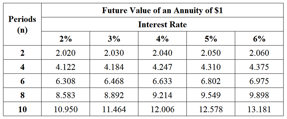
Use the table below to justify your answer. (2 marks)

--- 4 WORK AREA LINES (style=lined) ---

Show Answers Only

`text(Dominique will not have saved)`

`text(enough to reach)\ $15\ 000.`

Show Worked Solution

`text(Interest rate)\ text{(6 monthly)} = text(4%) -: 2 = text(2%)`

`n = 4\ \ \ text{(6 month periods in 2 years)}`

`=>\ text(FVA factor) = 4.122\ \ \ text{(from Table)}`

`text(FVA)= 3500 xx 4.122= $14\ 427`

`:.\ text(Dominique will not have saved enough to)`

`text(reach)\ $15\ 000.`

Financial Maths, STD2 F5 EQ-Bank 30

Camilla buys a car for $21 000 and repays it over 4 years through equal monthly instalments.

She pays a 10% deposit and interest is charged at 9% p.a. on the reducing balance loan.

Using the Table of present value interest factors below, where `r` represents the monthly interest and `N` represents the number of repayments

Calculate the monthly repayment, `$P`, that Camilla must pay to complete the loan after 4 years (to the nearest $). (3 marks)

--- 6 WORK AREA LINES (style=lined) ---
Calculate the total interest paid over the life of the loan. (1 mark)

--- 1 WORK AREA LINES (style=lined) ---

Show Answers Only

a. `text(Camilla must repay $470 per month)`

b. `$3660`

Show Worked Solution

a. `text(Deposit) = 10text(%) xx 21\ 000 = $2100`

`text(Loan Value)= 21\ 000-2100= $18\ 900`

`text(Monthly interest rate) = text(9%)/12 = 0.0075`

`text(# Repayments) = 4 xx 12 = 48`

`=>\ text(PVA Factor) = 40.18478\ \ text{(from Table)}`

`text(Monthly repayment)\ ($P)`	`= (18\ 900)/(40.18478)`
	`= 470.32…= $470\ text{(nearest $)}`

`:.\ text(Camilla must repay $470 per month.)`

b. `text(Total Repayments)= 48 xx 470= $22\ 560`

`:.\ text(Interest paid over loan)= 22\ 560-18\ 900= $3660`

Statistics, STD2 S5 2008 HSC 28a

The following graph indicates `z`-scores of ‘height-for-age’ for girls aged 5 – 19 years.

What is the `z`-score for a six year old girl of height 120 cm? (1 mark)

--- 2 WORK AREA LINES (style=lined) ---
Rachel is 10 ½ years of age.

(1) If 2.5% of girls of the same age are taller than Rachel, how tall is she? (1 mark)

--- 1 WORK AREA LINES (style=lined) ---

(2) Rachel does not grow any taller. At age 15 ½, what percentage of girls of the same age will be taller than Rachel? (2 marks)

--- 4 WORK AREA LINES (style=lined) ---
What is the average height of an 18 year old girl? (1 mark)

--- 1 WORK AREA LINES (style=lined) ---

For adults (18 years and older), the Body Mass Index is given by

`B = m/h^2` where `m = text(mass)` in kilograms and `h = text(height)` in metres.

The medically accepted healthy range for `B` is `21 <= B <= 25`.

What is the minimum weight for an 18 year old girl of average height to be considered healthy? (2 marks)

--- 4 WORK AREA LINES (style=lined) ---
The average height, `C`, in centimetres, of a girl between the ages of 6 years and 11 years can be represented by a line with equation

`C = 6A + 79` where `A` is the age in years.

(1) For this line, the gradient is 6. What does this indicate about the heights of girls aged 6 to 11? (1 mark)

--- 2 WORK AREA LINES (style=lined) ---

(2) Give ONE reason why this equation is not suitable for predicting heights of girls older than 12. (1 mark)

--- 2 WORK AREA LINES (style=lined) ---

Show Answers Only

`1`
(1) `155\ text(cm)`

(2) `text(84%)`
`163\ text(cm)`
`55.8\ text(kg)`
(1) `text(It indicates that 6-11 year old girls)`

`text(grow, on average, 6cm per year)`

(2) `text(Girls eventually stop growing, and the)`

`text(equation doesn’t factor this in.)`

Show Worked Solution

i.	`z text(-score) = 1`

ii.	(1)	`text(If 2 ½ % are taller than Rachel)`
		`=> z text(-score of +2)`
		`:.\ text(She is 155 cm)`

	(2)	`text(At age)\ 15\ ½,\ 155\ text(cm has a)\ z text(-score of –1)`
		`text(68% between)\ z = 1\ text(and)\ –1`
		`=> text(34% between)\ z = 0\ text(and)\ –1`
		`text(50% have)\ z >= 0`

		`:.\ text(% Above)\ z text(-score of –1)`
		`= 50 + 34`
		`= 8text(4%)`

`:.\ text(84% of girls would be taller than Rachel at age)\ 15 ½.`

iii.	`text(Average height of 18 year old has)\ z text(-score = 0)`
	`:.\ text(Average height) = 163\ text(cm)`

iv.	`B = m/h^2`
	`h = 163\ text(cm) = 1.63\ text(m)`

`text(Given)\ \ 21 <= B <= 25,\ text(minimum healthy)`

`text(weight occurs when)\ B = 21`

`=> 21`	`= m/1.63^2`
`m`	`= 21 xx 1.63^2`
	`= 55.794…`
	`= 55.8\ text(kg)\ text{(1 d.p.)}`

v.	(1)	`text(It indicates that 6-11 year old girls, on average, grow)`
		`text(6 cm per year.)`
	(2)	`text(Girls eventually stop growing, and the equation doesn’t)`
		`text(factor this in.)`

Statistics, STD2 S1 2008 HSC 26d

The graph shows the predicted population age distribution in Australia in 2008.

How many females are in the 0–4 age group? (1 mark)

--- 1 WORK AREA LINES (style=lined) ---
What is the modal age group? (1 mark)

--- 1 WORK AREA LINES (style=lined) ---
How many people are in the 15–19 age group? (2 marks)

--- 4 WORK AREA LINES (style=lined) ---
Give ONE reason why there are more people in the 80+ age group than in the 75–79 age group. (1 mark)

--- 2 WORK AREA LINES (style=lined) ---

Show Answers Only

a. `600\ 000`

b. `35-39`

c. `1\ 450\ 000`

d. `text(The 80+ group includes all people over 80)`

`text(and is not restricted by a 5-year limit.)`

Show Worked Solution

a. `text{# Females} (0-4)= 0.6 xx 1\ 000\ 000= 600\ 000`

b. `text(Modal age group)\ =35-39`

c. `text{# Males} (15-19)= 0.75 xx 1\ 000\ 000= 750\ 000`

`text{# Females} (15-19)= 0.7 xx 1\ 000\ 000= 700\ 000`

`:.\ text{Total People} (15-19)`	`= 750\ 000 + 700\ 000`
	`= 1\ 450\ 000`

d.	`text(The 80+ group includes all people over 80)`
	`text(and is not restricted by a 5-year limit.)`

Probability, STD2 S2 2008 HSC 26b

The retirement ages of two million people are displayed in a table.

What is the relative frequency of the 51–55 year retirement age? (1 mark)

--- 1 WORK AREA LINES (style=lined) ---
Describe the distribution. (1 mark)

--- 2 WORK AREA LINES (style=lined) ---

Show Answers Only

a. `7/400`

b. `text(Distribution is negatively skewed because as age increases, so does the)`

`text(number of people in each age bracket.)`

Show Worked Solution

a. `text(Relative frequency)\ (51-55)`

`= text{# People (51-55)}/text(Total People)`

`= (35\ 000)/(2\ 000\ 000)= 7/400`

b. `text(Distribution is negatively skewed because as age increases, so does the)`

`text(number of people in each age bracket.)`

Probability, STD2 S2 2008 HSC 26a

Cecil invited 175 movie critics to preview his new movie. After seeing the movie, he conducted a survey. Cecil has almost completed the two-way table.

Determine the value of `A`. (1 mark)

--- 1 WORK AREA LINES (style=lined) ---
A movie critic is selected at random.

What is the probability that the critic was less than 40 years old and did not like the movie? (2 marks)

--- 4 WORK AREA LINES (style=lined) ---
Cecil believes that his movie will be a box office success if 65% of the critics who were surveyed liked the movie.

Will this movie be considered a box office success? Justify your answer. (1 mark)

--- 2 WORK AREA LINES (style=lined) ---

Show Answers Only

a. `58`

b. `6/25`

c. `text(Proof)\ \ text{(See Worked Solutions)}`

Show Worked Solution

a. `text{Critics liked and}\ >= 40 = 102-65 = 37`

`A = 37+31=68`

b. `text{Critics did not like and < 40} = 175-65-37-31= 42`

`P text{(not like and < 40)}= 42/175= 6/25`

c. `text(Critics liked) = 102`

`text(% Critics liked)= 102/175 xx 100= 58.28…%`

`:.\ text{Movie NOT a box office success (< 65% critics liked)}`

Statistics, STD2 S1 2008 HSC 23f

Christina has completed three Mathematics tests. Her mean mark is 72%.

What mark (out of 100) does she have to get in her next test to increase her mean mark to 73%? (2 marks)

--- 5 WORK AREA LINES (style=lined) ---

Show Answers Only

`76`

Show Worked Solution

`text(Total marks in 3 tests)= 3 xx 72= 216`

`text(We need 4-test mean) = 73`

`text{i.e. Total Marks (4 tests)}-:4= 73`

`text(Total Marks)\ text{(4 tests)}= 292`

`:.\ text(4th test score)= 292-216= 76`

Statistics, STD2 S1 2008 HSC 23e

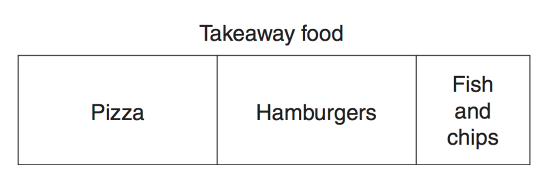
In a survey, 450 people were asked about their favourite takeaway food. The results are displayed in the bar graph.

How many people chose pizza as their favourite takeaway food? (2 marks)

Show Answers Only

`175`

Show Worked Solution

`text(Number of people who chose pizza)`

COMMENT: This question required measurement of the actual image on the exam. The same methodology works here.

`= text{Length of pizza section}/text{Total length of bar} xx 450`

`~~ 7/18 xx 450~~ 175`

`:.\ 175\ text(people chose pizza.)`

Measurement, STD2 M6 2008 HSC 17 MC

The diagram shows the position of `Q`, `R` and `T` relative to `P`.

In the diagram,

`Q` is south-west of `P`

`R` is north-west of `P`

`/_QPT` is 165°

What is the bearing of `T` from `P`?

`060^@`
`075^@`
`105^@`
`120^@`

Show Answers Only

`A`

Show Worked Solution

`/_QPS=45^@\ \ \ text{(} Q\ text(is south west of)\ Ptext{)}`

`/_TPS = 165-45 = 120^@`

`:.\ /_NPT = 60^@\ \ text{(} 180^@\ text(in straight line)text{)}`

`=> A`

Statistics, STD2 S1 2008 HSC 13 MC

The height of each student in a class was measured and it was found that the mean height was 160 cm.

Two students were absent. When their heights were included in the data for the class, the mean height did not change.

Which of the following heights are possible for the two absent students?

155 cm and 162 cm
152 cm and 167 cm
149 cm and 171 cm
143 cm and 178 cm

Show Answers Only

`C`

Show Worked Solution

`text(S) text(ince the mean doesn’t change)`

`=>\ text(2 absent students must have a)`

`text(mean height of 160 cm.)`

`text(Considering each option given,)`

`(149 + 171) -: 2 = 160`

`=> C`

Statistics, STD2 S4 2008 HSC 12 MC

A scatterplot is shown.

Which of the following best describes the correlation between $R$ and $T$?

Positive
Negative
Positively skewed
Negatively skewed

Show Answers Only

$A$

Show Worked Solution

$\text{Correlation is positive.}$

$\text{NB. The skew does not directly relate to correlation.}$

$\Rightarrow A$

Statistics, STD2 S1 2008 HSC 10 MC

The marks for a Science test and a Mathematics test are presented in box-and-whisker plots.

Which measure must be the same for both tests?

Mean
Range
Median
Interquartile range

Show Answers Only

`D`

Show Worked Solution

`text(IQR)=text(Upper Quartile)-text(Lower Quartile)`

`text{In both box plots, IQR = 3 intervals (against bottom scale)}`

`=> D`

Statistics, STD2 S1 2008 HSC 8 MC

What is the median of the following set of scores?

Show Answers Only

`C`

Show Worked Solution

`text(Median)=(n+1)/2=(33+1)/2=\ text (17th score)`

`:.\ text(Median is 14)`

`=> C`

Statistics, STD2 S1 2008 HSC 3 MC

The stem-and-leaf plot represents the daily sales of soft drink from a vending machine.

If the range of sales is 43, what is the value of

Show Answers Only

`A`

Show Worked Solution

`text(Range = High) – text(Low) = 43`

`:.\ 67 – text(Low)`	`= 43`
`text(Low)`	`= 24`

`:.\ N = 4`

`=> A`

Functions, 2ADV F1 2008 HSC 1c

Simplify `2/n-1/(n+1)`. (2 marks)

--- 4 WORK AREA LINES (style=lined) ---

Show Answers Only

`(n + 2)/(n(n+1))`

Show Worked Solution

`2/n-1/(n+1)`

`= (2(n+1)-1(n))/(n(n+1))`

`= (2n + 2-n)/(n(n+1))`

`= (n+2)/(n(n+1))`

Financial Maths, STD2 F5 EQ-Bank 22

The table below shows the present value of an annuity with a contribution of $1.

Fiona pays $3000 into an annuity at the end of each year for 4 years at 2% p.a., compounded annually. What is the present value of her annuity? (1 mark)

--- 2 WORK AREA LINES (style=lined) ---
If John pays $6000 into an annuity at the end of each year for 2 years at 4% p.a., compounded annually, is he better off than Fiona? Use calculations to justify your answer. (2 marks)

--- 4 WORK AREA LINES (style=lined) ---

Show Answers Only

a. `$11\ 423.10`

b. `text(Proof)\ \ text{(See Worked Solutions)}`

Show Worked Solution

a. `text(Table factor when)\ \ n = 4,\ r = text(2%) \ => \ 3.8077`

`:.\ PVA\ text{(Fiona)}= 3000 xx 3.8077= $11\ 423.10`

b. `text(Table factor when)\ n = 2, r = text(4%)`

`=> 1.8861`

`:.\ PVA\ text{(John)}= 6000 xx 1.8861= $11\ 316.60`

`:.\ text(Fiona will be better off because her)\ PVA`

`text(is higher.)`

Trigonometry, 2ADV T1 2014 HSC 13d

Chris leaves island `A` in a boat and sails 142 km on a bearing of 078° to island `B`. Chris then sails on a bearing of 191° for 220 km to island `C`, as shown in the diagram.

Show that the distance from island `C` to island `A` is approximately 210 km. (2 marks)

--- 5 WORK AREA LINES (style=lined) ---
Chris wants to sail from island `C` directly to island `A`. On what bearing should Chris sail? Give your answer correct to the nearest degree. (3 marks)

--- 9 WORK AREA LINES (style=lined) ---

Show Answers Only

`text(Proof)\ \ text{(See Worked Solutions)}`
`333°`

Show Worked Solution

`text(Find)\ \ /_ABC`

`text(Let)\ D\ text(be south of)\ B`

`:.\ /_CBD = 191-180 = 11°`

`/_ DBA`	`= 78°\ text{(alternate)}`
`/_ ABC`	`= 78-11= 67°`

`text(Using Cosine rule:)`

`AC^2`	`= AB^2 + BC^2-2 * AB * BC * cos /_ABC`
	`= 142^2 + 220^2-2 xx 142 xx 220 xx cos 67°`
	`= 44\ 151.119…`
`AC`	`= 210.121…~~ 210\ text(km)\ \ \ text(… as required)`

ii. `text(Find)\ \ /_ ACB`

`text(Using Sine rule:)`

`(sin /_ ACB)/142`	`= (sin /_ABC)/210`
`sin /_ ACB`	`= (142 xx sin 67°)/210= 0.6224…`
`/_ ACB`	`= 38.494…= 38°\ text{(nearest degree)}`

`text(Let)\ E\ text(be due North of)\ C`

`/_ECB = 11°\ text{(} text(alternate to)\ /_CBD text{)}`

`/_ECA= 38-11= 27°`

`:.\ text(Bearing of)\ A\ text(from)\ C`

`= 360-27`

`= 333°`

Statistics, STD2 S4 2014* HSC 30b

The scatterplot shows the relationship between expenditure per primary school student, as a percentage of a country’s Gross Domestic Product (GDP), and the life expectancy in years for 15 countries.

For the given data, the correlation coefficient, `r`, is 0.83. What does this indicate about the relationship between expenditure per primary school student and life expectancy for the 15 countries? (1 mark)

--- 1 WORK AREA LINES (style=lined) ---
For the data representing expenditure per primary school student, `Q_L` is 8.4 and `Q_U` is 22.5.

What is the interquartile range? (1 mark)

--- 1 WORK AREA LINES (style=lined) ---
Another country has an expenditure per primary school student of 47.6% of its GDP.

Would this country be an outlier for this set of data? Justify your answer with calculations. (2 marks)

--- 4 WORK AREA LINES (style=lined) ---
On the scatterplot, draw the least-squares line of best fit `y = 1.29x + 49.9`. (2 marks)

--- 4 WORK AREA LINES (style=lined) ---
Using this line, or otherwise, estimate the life expectancy in a country which has an expenditure per primary school student of 18% of its GDP. (1 mark)

--- 1 WORK AREA LINES (style=lined) ---
Why is this line NOT useful for predicting life expectancy in a country which has expenditure per primary school student of 60% of its GDP? (1 mark)

--- 1 WORK AREA LINES (style=lined) ---

Show Answers Only

a. `text(It indicates there is a strong positive)`

`text(correlation between the two variables.)`

b. `14.1`

c. `text(Yes, because it’s > 43.65%)`

e. `73.1\ text(years)`

f. `text(At 60% GDP, the line predicts a life expectancy)`

`text(of 127.3. This line of best fit is only accurate)`

`text(in a lower range of GDP expenditure.)`

Show Worked Solution

a. `text(It indicates there is a strong positive)`

`text(correlation between the two variables)`

b.	`text(IQR)`	`= Q_U\-Q_L`
		`= 22.5\-8.4= 14.1`

♦ Mean mark (c) 35%

c. `text(An outlier on the upper side must be more than)`

`Q_u\ +1.5xxIQR`

`=22.5+(1.5xx14.1)`

`=\ text(43.65%)`

`:.\ text(A country with an expenditure of 47.6% is an outlier).`

e. `text(Life expectancy) ~~ 73.1\ text{years (see dotted line)}`

♦♦ Mean mark (e) 39%

`text(Alternative Solution)`

`text(When)\ x=18`

`y=1.29(18)+49.9=73.12\ \ text(years)`

♦♦♦ Mean mark (f) 0%. The toughest question on the 2014 paper.
COMMENT: Examiners regularly ask students to identify and comment on outliers where linear relationships break down.

f. `text(At 60% GDP, the line predicts a life expectancy)`

`text(of 127.3. This line of best fit is only accurate)`

`text(in a lower range of GDP expenditure.)`

Financial Maths, STD2 F4 2014 HSC 30a

Chandra and Sascha plan to have $20 000 in an investment account in 15 years time for their grandchild’s university fees.

The interest rate for the investment account will be fixed at 3% per annum compounded monthly.

Calculate the amount that they will need to deposit into the account now in order to achieve their plan. (3 marks)

--- 6 WORK AREA LINES (style=lined) ---

Show Answers Only

`$12\ 760\ \ text{(nearest $)}`

Show Worked Solution

♦ Mean mark 49%

`FV = $20\ 000,\ \ n = 15xx 12=180,`

`r = 0.03 /12=0.0025`

`FV`	`= PV (1 + r)^n`
`20\ 000`	`=PV (1 + 0.0025)^180`
`PV`	`=(20\ 000)/(1.0025)^180`
	`=$12\ 759.73…`

`:.\ text(They need to deposit) \ \ $12\ 760\ \ text{(nearest $)}`

Statistics, STD2 S1 2014 HSC 29c

Terry and Kim each sat twenty class tests. Terry’s results on the tests are displayed in the box-and-whisker plot shown in part (i).

Kim’s 5-number summary for the tests is 67, 69, 71, 73, 75.

Draw a box-and-whisker plot to display Kim’s results below that of Terry’s results. (1 mark)
What percentage of Terry’s results were below 69? (1 mark)

--- 1 WORK AREA LINES (style=lined) ---
Terry claims that his results were better than Kim’s. Is he correct?

Justify your answer by referring to the summary statistics and the skewness of the distributions. (4 marks)

--- 8 WORK AREA LINES (style=lined) ---

Show Answers Only

a. `text(See Worked Solutions)`

b. `text(50%)`

c. `text(See Worked Solutions)`

Show Worked Solution

♦ Mean mark (b) 39%

b. `text(50%)`

c. `text(Terry’s results are more positively skewed than)`

♦♦ Mean mark 29%
COMMENT: Examiners look favourably on using language of location in answers, particularly the areas they have specifically pointed students towards (skewness in this example).

`text(Kim’s and also have a higher limit high.)`

`text(However, Kim’s results are more consistent,)`

`text(showing a tighter IQR. They also have a)`

`text(significantly higher median than Terry’s and)`

`text(are evenly skewed.)`

`:.\ text(Kim’s results were better.)`

Statistics, STD2 S1 2014 HSC 26e

The times taken for 160 music downloads were recorded, grouped into classes and then displayed using the cumulative frequency histogram shown.

On the diagram, draw the lines that are needed to find the median download time. (2 marks)

--- 0 WORK AREA LINES (style=lined) ---

Show Answers Only

Show Worked Solution

♦♦♦ Mean mark 17%.

Algebra, STD2 A1 2014 HSC 26c

Solve the equation `(5x + 1)/3-4 = 5-7x`. (3 marks)

Show Answers Only

`x = 1`

Show Worked Solution

`(5x + 1)/3-4`	`= 5-7x`
`5x + 1-3(4)`	`= 3(5-7x)`
`5x + 1-12`	`= 15-21x`
`26x`	`= 26`
`:. x`	`= 1`

Statistics, STD2 S5 2014 HSC 24 MC

The weights of 10 000 newborn babies in NSW are normally distributed. These weights have a mean of 3.1 kg and a standard deviation of 0.35 kg.

How many of these newborn babies have a weight between 2.75 kg and 4.15 kg?

`4985`
`6570`
`8370`
`8385`

Show Answers Only

`D`

Show Worked Solution

♦ Mean mark 46%

`text(Find)\ z text(-scores of 2.75 and 4.15 kg)`

`z\ (2.75)`	`= (x-mu)/5 = (2.75-3.1)/0.35 = -1`
`z\ (4.15)`	`= (4.15-3.1)/0.35 = 3`

`text(68% between)\ z=–1\ text(and 1)\ => \ text(34% between)\ z=–1\ text(and 0)`

`text(99.7% between)\ z=–3\ text(and 3) \ => \ text(49.85% between)\ z=0\ text(and)\ 3`

`%\ text(with)\ z text(-scores between)\ –1\ text(and 3) = 34 + 49.85 =\ text(83.85%)`

`text(Babies between 2.75 kg and 4.15 kg) = text(83.85%) xx 10\ 000 = 8385`

`=> D`

Measurement, STD2 M6 2014 HSC 23 MC

The following information is given about the locations of three towns `X`, `Y` and `Z`:

• `X` is due east of `Z`

• `X` is on a bearing of 145° from `Y`

• `Y` is on a bearing of 060° from `Z`.

Which diagram best represents this information?

Show Answers Only

`C`

Show Worked Solution

♦ Mean mark 38%
COMMENT: Drawing a parallel North/South line through `Y` makes this question much simpler to solve.

`text(S)text(ince)\ X\ text(is due east of)\ Z`

`=> text(Cannot be)\ B\ text(or)\ D`

`text(The diagram shows we can find)`

`/_ZYX = 60 + 35^@ = 95^@`

`text(Using alternate angles)\ (60^@)\ text(and)`

`text(the)\ 145^@\ text(bearing of)\ X\ text(from)\ Y`

`=> C`

Financial Maths, STD2 F5 2014 HSC 21 MC

A table of future value interest factors is shown.

A certain annuity involves making equal contributions of `$25 000` into an account every 6 months for 2 years at an interest rate of 4% per annum.

Based on the information provided, what is the future value of this annuity?

`$50\ 500`
`$51\ 000`
`$103\ 040`
`$106\ 162`

Show Answers Only

`C`

Show Worked Solution

`text(4 contributions of $25 000 made.)`

♦ Mean mark 43%

`text(Annuity period = 6 months)`

`text{Rate (per annuity period)}=(text(4%))/2=text(2%)`

`text{No. Periods = 4 (4 x 6 months = 2 years)}`

`text(Table value = 4.1216)`

`:.\ text(Annuity Value)=4.1216 xx 25\ 000=$103\ 040`

`=> C`

Statistics, STD2 S1 2014 HSC 14 MC

Twenty Year 12 students were surveyed. These students were asked how many hours of sport they play per week, to the nearest hour.

The results are shown in the frequency table.

\begin{array} {|c|c|}
\hline
\rule{0pt}{2.5ex} \textit{Hours per week} \rule[-1ex]{0pt}{0pt} & \ \ \ \ \ \textit{Frequency}\ \ \ \ \ \\
\hline
\rule{0pt}{2.5ex} 0-2 \rule[-1ex]{0pt}{0pt} & 5 \\
\hline
\rule{0pt}{2.5ex} 3-5 \rule[-1ex]{0pt}{0pt} & 10 \\
\hline
\rule{0pt}{2.5ex} 6-8 \rule[-1ex]{0pt}{0pt} & 3 \\
\hline
\rule{0pt}{2.5ex} 9-11 \rule[-1ex]{0pt}{0pt} & 2 \\
\hline
\end{array}

What is the mean number of hours of sport played by the students per week?

Show Answers Only

$B$

Show Worked Solution

$\text{Using the class centres}$

$\text{Total hours}$	$=(1\times 5) + (4\times 10) + (7\times 3) + (10\times 2)$
	$= 5 + 40 + 21 + 20= 86$

♦ Mean mark 45%
COMMENT: The mean is calculated using “class centres” in grouped data.

$\text{Mean hours}=\dfrac{86}{20} =4.3$

$\Rightarrow B$

Probability, STD2 S2 2014 HSC 8 MC

A group of 150 people was surveyed and the results recorded.

A person is selected at random from the surveyed group.

What is the probability that the person selected is a male who does not own a mobile?

`28/150`
`45/150`
`28/70`
`45/70`

Show Answers Only

`A`

Show Worked Solution

`P=text(number of males without mobile)/text(number in group)= 28/150`

`=> A`

Functions, 2ADV F1 2009 HSC 1a

Sketch the graph of `y-2x = 3`, showing the intercepts on both axes. (2 marks)

--- 8 WORK AREA LINES (style=lined) ---

Show Answers Only

Show Worked Solution

`y-2x=3\ \ =>\ \ y=2x+3`

`ytext{-intercept}\ = 3`

`text{Find}\ x\ text{when}\ y=0:`

`0-2x=3\ \ =>\ \ x=-3/2`

Financial Maths, STD2 F5 2011 HSC 27d

Josephine invests $50 000 for 15 years, at an interest rate of 6% per annum, compounded annually.

Emma invests $500 at the end of each month for 15 years, at an interest rate of 6% per annum, compounded monthly.

Financial gain is defined as the difference between the final value of an investment and the total contributions.

Who will have the better financial gain after 15 years? Using the Table below* and appropriate formulas, justify your answer with suitable calculations. (4 marks)

--- 8 WORK AREA LINES (style=lined) ---

Show Answers Only

`text(Josephine – see Worked Solutions)`

Show Worked Solution

♦ Mean mark 42%
COMMENT: Note that compound interest vs annuity comparisons are commonly tested.

`text(Josephine)`

`text(Investment)`	`= 50\ 000 (1 + 0.06)^15`
	`= 50\ 000 (1.06)^15= $119\ 827.91`

`text(Financial gain)= 119\ 827.91-50\ 000= $69\ 827.91`

`text(Emma)`

`text{Monthly interest rate} = text(6%)-:12=text(0.5%)`

`text{# Monthly Payments}=12 xx 15=180`

`=>\ text{Annuity Factor = 290.8187 (from Table)}`

`text(Investment)= 500 xx 290.8187= $145\ 409.35`

`text(Financial gain)`	`= 145\ 409.35\-text(total contributions)`
	`= 145\ 409.35\-(500 xx 12 xx 15)`
	`= 145\ 409.35\-90\ 000= $55\ 409.35`

`:.\ text(Josephine will have the better financial gain.)`

Statistics, STD2 S5 2011 HSC 27c

Two brands of light bulbs are being compared. For each brand, the life of the light bulbs, in hours, is normally distributed and described in the table below.

\begin{array} {|l|c|c|}
\hline
\rule{0pt}{2.5ex} \rule[-1ex]{0pt}{0pt} & \quad \text{Mean} \quad & \text{Standard Deviation} \\
\hline
\rule{0pt}{2.5ex} \text{Brand A} \rule[-1ex]{0pt}{0pt} & 450 & 25 \\
\hline
\rule{0pt}{2.5ex} \text{Brand B} \rule[-1ex]{0pt}{0pt} & 500 & 50 \\
\hline
\end{array}

One of the Brand B light bulbs has a life of 400 hours.
What is the `z`-score of the life of this light bulb? (1 mark)

--- 1 WORK AREA LINES (style=lined) ---
A light bulb is considered defective if it lasts less than 400 hours. The following claim is made:
‘Brand A light bulbs are more likely to be defective than Brand B light bulbs.’
Is this claim correct? Justify your answer, with reference to `z`-scores or standard deviations or the normal distribution. (2 marks)
--- 4 WORK AREA LINES (style=lined) ---

Show Answers Only

a. `-2`

b. `text(The claim is incorrect.)`

Show Worked Solution

a. `z text{-score of Brand B bulb (400 hrs)}`

`= (x-mu)/sigma= (400-500)/50= -2`

b. `z text{-score of Brand A bulb (400 hours)}`

♦ Mean mark (b) 42%

`=(400-450)/25=-2`

`text(S)text(ince the)\ z text(-score for both brands is –2, they are equally likely to be defective.)`

`:.\ text(The claim is incorrect.)`

Statistics, STD2 S1 2011 HSC 25d

Data was collected from 30 students on the number of text messages they had sent in the previous 24 hours. The set of data collected is displayed.

What is the outlier for this set of data? (1 mark)

--- 1 WORK AREA LINES (style=lined) ---
What is the interquartile range of the data collected from the female students? (1 mark)

--- 1 WORK AREA LINES (style=lined) ---

Show Answers Only

a. `71`

b. `9`

Show Worked Solution

a. `text(Outlier is 71)`

♦♦ Mean mark 34%
COMMENT: Ensure you can quickly and accurately find quartile values using stem and leaf graphs!

b. `text{Lower quartile = 11 (4th female data point)}`

`text{Upper quartile = 20 (11th female data point)}`

`:.\ text{Interquartile range (female)}=20-11=9`

Probability, STD2 S2 2011 HSC 25c

At another school, students who use mobile phones were surveyed. The set of data is shown in the table.

How many students were surveyed at this school? (1 mark)

--- 1 WORK AREA LINES (style=lined) ---
Of the female students surveyed, one is chosen at random. What is the probability that she uses pre-paid? (1 mark)

--- 2 WORK AREA LINES (style=lined) ---

Ten new male students are surveyed and all ten are on a plan. The set of data is updated to include this information.

What percentage of the male students surveyed are now on a plan? Give your answer to the nearest per cent. (1 mark)

--- 2 WORK AREA LINES (style=lined) ---

Show Answers Only

a. `580`

b. `text(54%)`

c. `text(42%)`

Show Worked Solution

a. `text(# Students surveyed)=319+261=580`

b. `Ptext{(Female uses prepaid)}`

`=text(# Females on prepaid)/text(Total females)=172/319=0.53918… ~~ 54\text{% (nearest %)}`

c. `text(% Males on plan)`	`=text(# Males on plan + 10)/text(Total males + 10)=(103+10)/(261+10)`
	`=113/271=0.4169…=42\text{% (nearest %)}`

Statistics, STD2 S1 2011 HSC 25b

The graph below displays data collected at a school on the number of students
in each Year group, who own a mobile phone.

Which Year group has the highest percentage of students with mobile phones? (1 mark)

--- 1 WORK AREA LINES (style=lined) ---
Two students are chosen at random, one from Year 9 and one from Year 10.

Which student is more likely to own a mobile phone?

Justify your answer with suitable calculations. (2 marks)

--- 4 WORK AREA LINES (style=lined) ---
Identify a trend in the data shown in the graph. (1 mark)

--- 2 WORK AREA LINES (style=lined) ---

Show Answers Only

a. `text{Year 12 (100%)}`

b. `text(Year 10)`

c. `text(See Worked Solutions for detail)`

Show Worked Solution

a. `text(Year 12 (100%))`

MARKER’S COMMENT: Many students ignore the instruction to use calculations and lose marks as a result.

b.	`text(% Ownership in Year 9)`	`=55/70`
		`=\ text{78.6% (1d.p.)}`
	`text(% Ownership in Year 10)`	`=50/60`
		`=\ text{83.3% (1d.p.)}`

`:.\ text(The Year 10 student is more likely to own a mobile phone.)`

c. `text(% Ownership increases as students)`

`text(progress from Year 7 to Year 12.)`

Statistics, STD2 S1 2011 HSC 25a

A study on the mobile phone usage of NSW high school students is to be conducted.

Data is to be gathered using a questionnaire.

The questionnaire begins with the three questions shown.

Classify the type of data that will be collected in Q2 of the questionnaire. (1 mark)

--- 1 WORK AREA LINES (style=lined) ---
Write a suitable question for this questionnaire that would provide discrete ordinal data. (1 mark)

--- 2 WORK AREA LINES (style=lined) ---
An initial study is to be conducted using a stratified sample.

Describe a method that could be used to obtain a representative stratified sample. (1 mark)

--- 2 WORK AREA LINES (style=lined) ---
Who should be surveyed if it is decided to use a census for the study? (1 mark)

--- 2 WORK AREA LINES (style=lined) ---

Show Answers Only

a. `text(Categorical)`

b. `text(See Worked Solutions)`

c. `text(See Worked Solutions)`

d. `text(A census would involve all high school students in NSW.)`

Show Worked Solution

a. `text(Categorical)`

b. `text(How often do you use your mobile phone each day?)`

`text{(Option structure:- Never, Rarely, Sometimes, Often, Always.)}`

c. `text(The method could be to work out how many)`

♦♦♦ Mean mark 7%.
COMMENT: Know random, systematic and stratified sampling definitions.

`text{students are in each year and ask 10% of the}`

`text{students in each year. (Note the sample of}`

`text{students in each year must be proportional to}`

`text{their percentage in the population).}`

♦♦♦ Mean mark 18%.
MARKER’S COMMENT: A specific population is required here.

d. `text(A census would involve all high school)`

`text(students in NSW.)`

Financial Maths, STD2 F4 2011 HSC 23c

An amount of $5000 is invested at 10% per annum, compounded six-monthly.

Use the table to find the value of this investment at the end of three years. (2 marks)

Show Answers Only

`$6700`

Show Worked Solution

♦♦ Mean mark 28%
MARKER’S COMMENT: Remember that the number of periods is the number of “compounding periods” and when asked to use the table, use the table!

`text(Interest rate)= text(10% pa)= text(5% per 6 months)`

`text(Period)= 6\ \ \ \ text{(6 x 6 months in 3 years)}`

`=> text(Table value)=1.340`

`:.\ text(Value of investment)`	`=5000xx1.34`
	`=$6700`

Algebra, STD2 A2 2010 HSC 27c

The graph shows tax payable against taxable income, in thousands of dollars.

2010 27c

Use the graph to find the tax payable on a taxable income of $21 000. (1 mark)

--- 1 WORK AREA LINES (style=lined) ---
Use suitable points from the graph to show that the gradient of the section of the graph marked `A` is `1/3`. (1 mark)

--- 3 WORK AREA LINES (style=lined) ---
How much of each dollar earned between $21 000 and $39 000 is payable in tax? (1 mark)

--- 2 WORK AREA LINES (style=lined) ---
Write an equation that could be used to calculate the tax payable, `T`, in terms of the taxable income, `I`, for taxable incomes between $21 000 and $39 000. (2 marks)

--- 4 WORK AREA LINES (style=lined) ---

Show Answers Only

`$3000\ \ \ text{(from graph)}`
`1/3`
`33 1/3\ text(cents per dollar earned)`
`text(Tax payable on)\ I = 1/3 I\-4000`

Show Worked Solution

`text(Income on)\ $21\ 000=$3000\ \ \ text{(from graph)}`

b. `text(Using the points)\ (21,3)\ text(and)\ (39,9)`

♦♦ Mean mark 25%

`text(Gradient at)\ A`	`= (y_2-y_1)/(x_2-x_1)`
	`= (9000-3000)/(39\ 000-21\ 000)`
	`= 6000/(18\ 000)`
	`= 1/3\ \ \ \ \ text(… as required)`

c. `text(The gradient represents the tax applicable to each dollar)`

♦♦♦ Mean mark 12%!
MARKER’S COMMENT: Interpreting gradients is consistently asked and poorly answered.

`text(Tax)`	` = 1/3\ text(of each dollar earned)`
	` = 33 1/3\ text(cents per dollar earned)`

d. `text( Tax payable up to $21 000 = $3000)`

`text(Tax payable on income between $21 000 and $39 000)`

♦♦♦ Mean mark 15%.
STRATEGY: Earlier parts of a question provide important clues for devising an efficient solution strategy.

` = 1/3 (I-21\ 000)`

`:.\ text(Tax payable on)\ \ I`	`= 3000 + 1/3 (I-21\ 000)`
	`= 3000 + 1/3 I-7000`
	`= 1/3 I-4000`

Statistics, STD2 S1 2010 HSC 27b

The graphs show the distribution of the ages of children in Numbertown in 2000 and 2010.

In 2000 there were 1750 children aged 0–18 years.

How many children were aged 12–18 years in 2000? (1 mark)

--- 1 WORK AREA LINES (style=lined) ---
The number of children aged 12–18 years is the same in both 2000 and 2010.

How many children aged 0–18 years are there in 2010? (1 mark)

--- 1 WORK AREA LINES (style=lined) ---
Identify TWO changes in the distribution of ages between 2000 and 2010. In your answer, refer to measures of location or spread or the shape of the distributions. (2 marks)

--- 5 WORK AREA LINES (style=lined) ---
What would be ONE possible implication for government planning, as a consequence of this change in the distribution of ages? (1 mark)

--- 2 WORK AREA LINES (style=lined) ---

Show Answers Only

a. `875`

b. `3500`

c. `text{Changes in distribution (include 2 of the following):}`

`text(the lower quartile age is lower in 2010)`
`text(the median is lower in 2010)`
`text(the upper quartile age is lower in 2010)`
`text(the interquartile range is greater in 2010)`
`text(2010 is positively skewed while 2000 is negatively)`

d. `text(Implication for government planning:)`

`text(Since the children are getting younger in 2010,)`

`text(Approve and build more childcare facilities)`
`text(Build more school and public playgrounds)`

Show Worked Solution

a. `text{Since the median = 12 years}`

♦ Mean mark (a) 45%

`=>\ text{50% of children are aged 12–18 years}`

`:.\ text{Children aged 12–18}\ = 50\text{%}\ xx 1750 = 875`

♦♦ Mean mark (b) 25%

b. `text{Upper quartile (2010) = 12 years}`

`text{Children in upper quartile = 875 (from part (i))}`

`:.\ text{Children aged 0–18}\ =4 xx 875= 3500`

c. `text{Changes in distribution (include 2 of the following):}`

♦ Mean mark (c) 35%
MARKER’S COMMENT: A number of students incorrectly identified “positive” skew as “negative” skew here.

`text(the lower quartile age is lower in 2010)`
`text(the median is lower in 2010)`
`text(the upper quartile age is lower in 2010)`
`text(the interquartile range is greater in 2010)`
`text(2010 is positively skewed while 2000 is negatively)`

d. `text(Implication for government planning:)`

♦ Mean mark (d) 46%
MARKER’S COMMENT: Answers should reflect the 1 mark allocation.

`text(Since the children are getting younger in 2010,)`

`text(Approve and build more childcare facilities)`
`text(Build more school and public playgrounds)`

Statistics, STD2 S1 2010 HSC 26b

A new shopping centre has opened near a primary school. A survey is conducted to determine the number of motor vehicles that pass the school each afternoon between 2.30 pm and 4.00 pm.

The results for 60 days have been recorded in the table and are displayed in the cumulative frequency histogram.

Find the value of Χ in the table. (1 mark)

--- 1 WORK AREA LINES (style=lined) ---
On the cumulative frequency histogram above, draw a cumulative frequency polygon (ogive) for this data. (1 mark)
Use your graph to determine the median. Show, by drawing lines on your graph, how you arrived at your answer. (1 mark)
Prior to the opening of the new shopping centre, the median number of motor vehicles passing the school between 2.30 pm and 4.00 pm was 57 vehicles per day.

What problem could arise from the change in the median number of motor vehicles passing the school before and after the opening of the new shopping centre?

Briefly recommend a solution to this problem. (2 marks)

--- 5 WORK AREA LINES (style=lined) ---

Show Answers Only

a. `15`

d. `text(Problems)`

`text(- increased traffic delays)`

`text(- increased danger to students leaving school)`

`text(Solutions)`

`text(- signpost alternative routes around school)`

`text(- decrease the speed limit in the area)`

Show Worked Solution

a. `X= 25-10= 15`

♦♦♦ Mean mark 18%
MARKER’S COMMENT: The ogive was poorly drawn with many students incorrectly joining the middle of each column rather than from corner to corner.

♦♦ Mean mark 25%
MARKER’S COMMENT: Many students did not “show by drawing lines on the graph” as the question asked.

c. `text(Median)\ ~~155`

♦ Mean mark 47%
MARKER’S COMMENT: Short answers were often the best. Be concise when you can.

d.	`text(Problems)`
	`text(- increased traffic delays)`
	`text(- increased danger to students leaving school)`

	`text(Solutions)`
	`text(- signpost alternative routes around school)`
	`text(- decrease the speed limit in the area)`

Probability, STD2 S2 2011 HSC 24b

A die was rolled 72 times. The results for this experiment are shown in the table.

\begin{array} {|c|c|}
\hline
\rule{0pt}{2.5ex} \textit{Number obtained} \rule[-1ex]{0pt}{0pt} & \textit{Frequency} \\
\hline
\rule{0pt}{2.5ex} \ 1 \rule[-1ex]{0pt}{0pt} & 16 \\
\hline
\rule{0pt}{2.5ex} \ 2 \rule[-1ex]{0pt}{0pt} & 11 \\
\hline
\rule{0pt}{2.5ex} \ 3 \rule[-1ex]{0pt}{0pt} & \textbf{A} \\
\hline
\rule{0pt}{2.5ex} \ 4 \rule[-1ex]{0pt}{0pt} & 8 \\
\hline
\rule{0pt}{2.5ex} \ 5 \rule[-1ex]{0pt}{0pt} & 12 \\
\hline
\rule{0pt}{2.5ex} \ 6 \rule[-1ex]{0pt}{0pt} & 15 \\
\hline
\end{array}

Find the value of `A`. (1 mark)

--- 1 WORK AREA LINES (style=lined) ---
What was the relative frequency of obtaining a 4. (1 mark)

--- 2 WORK AREA LINES (style=lined) ---
If the die was unbiased, which number was obtained the expected number of times? (1 mark)

--- 2 WORK AREA LINES (style=lined) ---

Show Answers Only

a. $10$

b. $\dfrac{1}{9}$

c. $5$

Show Worked Solution

a. $\text{Since die rolled 72 times:}$

$A=72-(16+11+8+12+15)=10$

♦ Mean mark 38%
IMPORTANT: Many students confused ‘relative frequency’ with ‘frequency’ and incorrectly answered 8.

b. $\text{Relative frequency of 4}=\dfrac{8}{72}=\dfrac{1}{9}$

c. $\text{Expected frequency of any number}=\dfrac{1}{6}\times 72=12$

$\therefore\ \text{5 was obtained the expected number of times.}$

Algebra, STD2 A4 2011 HSC 20 MC

A function centre hosts events for up to 500 people. The cost `C`, in dollars, for the centre
to host an event, where `x` people attend, is given by:

`C = 10\ 000 + 50x`

The centre charges $100 per person. Its income `I`, in dollars, is given by:

`I = 100x`

How much greater is the income of the function centre when 500 people attend an event, than its income at the breakeven point?

`$15\ 000`
`$20\ 000`
`$30\ 000`
`$40\ 000`

Show Answers Only

`C`

Show Worked Solution

♦ Mean mark 50%
COMMENT: Students can read the income levels directly off the graph to save time and then check with the equations given.

`text(When)\ x=500,\ I=100xx500=$50\ 000`

`text(Breakeven when)\ \ x=200\ \ \ text{(from graph)}`

`text(When)\ \ x=200,\ I=100xx200=$20\ 000`

`text(Difference)=50\ 000-20\ 000=$30\ 000`

`=> C`

Statistics, STD2 S1 2011 HSC 17 MC

The heights of the players in a basketball team were recorded as 1.8 m, 1.83 m, 1.84 m, 1.86 m and 1.92 m. When a sixth player joined the team, the average height of the players increased by 1 centimetre.

What was the height of the sixth player?

1.85 m
1.86 m
1.91 m
1.93 m

Show Answers Only

`C`

Show Worked Solution

`text(Old Mean)`	`=(1.8+1.83+1.84+1.86+1.92)-:5`
	`=9.25/5=1.85\ \ text(m)`

`text{S}text{ince the new mean = 1.86m (given)}`

`text(New Mean)`	`=text(Height of all 6 players) -: 6`
`:.1.86`	`=(9.25+h)/6\ \ \ \ (h\ text{= height of new player})`
`h`	`=(6xx1.86)-9.25=1.91\ \ text(m)`

`=> C`

Statistics, STD2 S1 2011 HSC 14 MC

A data set of nine scores has a median of 7.

The scores 6, 6, 12 and 17 are added to this data set.

What is the median of the data set now?

Show Answers Only

`B`

Show Worked Solution

`text(S)text(ince an even amount of scores are added below and)`

`text(above the existing median, it will not change.)`

`=>B`

Financial Maths, STD2 F5 2009 HSC 27a

The table shows the future value of a $1 annuity at different interest rates over different numbers of time periods.

What would be the future value of a `$5000` per year annuity at 3% per annum for 6 years, with interest compounding yearly? (1 mark)

--- 1 WORK AREA LINES (style=lined) ---
What is the value of an annuity that would provide a future value of `$407\ 100` after 7 years at 5% per annum compound interest? (1 mark)

--- 1 WORK AREA LINES (style=lined) ---
An annuity of $1000 per quarter is invested at 4% per annum, compounded quarterly for 2 years. What will be the amount of interest earned? (3 marks)

--- 6 WORK AREA LINES (style=lined) ---

Show Answers Only

a. `$32\ 342`

b. `$50\ 000`

c. `$285.70`

Show Worked Solution

a. `text(Table factor when)\ \ n = 6,\ \ \ r =\ 3text(%) \ => \ 6.4684`

`:.\ FV= 5000 xx 6.4684= $32\ 342`

b. `text(Table factor when)\ \ n = 7,\ \ \ r =\ text(5%)`

♦ Mean mark (b) 45%
MARKER’S COMMENT: A common error was to multiply $407 100 by 8.1420 rather than divide.

`=> 8.1420`

`text(Let)\ \ A = text(annuity)`

`FV= A xx 8.1420`

`A= (FV)/8.1420= (407\ 100)/8.1420= $50\ 000`

c. `n=8\ \ \ (text(8 quarters in 2 years) )`

♦♦ Mean mark (c) 31%
MARKER’S COMMENT: When questions asked for the interest paid on annuities, remember to subtract the total principal amounts contributed.

`r = text(4%)/4 =\ text{1% per quarter}`

`:.\ text(Table factor) => 8.2857`

`FV=1000 xx 8.2857=$8285.70`

`text(Interest)`	`= FV (text(annuity) )\-text(Principal)`
	`= 8285.70-(8 xx 1000)= $285.70`

`:.\ text(Interest earned is $285.70)`

Probability, STD2 S2 2009 HSC 28d

In an experiment, two unbiased dice, with faces numbered 1, 2, 3, 4, 5, 6 are rolled 18 times.

The difference between the numbers on their uppermost faces is recorded each time. Juan performs this experiment twice and his results are shown in the tables.

Juan states that Experiment 2 has given results that are closer to what he expected than the results given by Experiment 1.

Is he correct? Explain your answer by finding the sample space for the dice differences and using theoretical probability. (4 marks)

--- 8 WORK AREA LINES (style=lined) ---

Show Answers Only

`text{Juan is correct (See Worked Solutions)}`

Show Worked Solution

♦♦♦ Mean mark 7%.
MARKER’S COMMENT: This question guides students by asking for an explanation using the sample space for the dice differences.

`text(Sample space for dice differences:)`

`text(Juan is correct. The table shows Experiment 1 has greater total differences to the)`

`text(expected frequencies than Experiment 2)`

Statistics, STD2 S4 2009 HSC 28b

The height and mass of a child are measured and recorded over its first two years.

\begin{array} {|l|c|c|}
\hline \rule{0pt}{2.5ex} \text{Height (cm), } H \rule[-1ex]{0pt}{0pt} & \text{45} & \text{50} & \text{55} & \text{60} & \text{65} & \text{70} & \text{75} & \text{80} \\
\hline \rule{0pt}{2.5ex} \text{Mass (kg), } M \rule[-1ex]{0pt}{0pt} & \text{2.3} & \text{3.8} & \text{4.7} & \text{6.2} & \text{7.1} & \text{7.8} & \text{8.8} & \text{10.2} \\
\hline
\end{array}

This information is displayed in a scatter graph.

Describe the correlation between the height and mass of this child, as shown in the graph. (1 mark)

--- 2 WORK AREA LINES (style=lined) ---
A line of best fit has been drawn on the graph.

Find the equation of this line. (2 marks)

--- 4 WORK AREA LINES (style=lined) ---

Show Answers Only

a. `text(The correlation between height and)`

`text(mass is positive and strong.)`

b. `M = 0.23H-8`

Show Worked Solution

a. `text(The correlation between height and)`

♦ Mean mark (a) 48%.

`text(mass is positive and strong.)`

b. `text(Using)\ \ P_1(40, 1.2)\ \ text(and)\ \ P_2(80, 10.4)`

♦♦♦ Mean mark (b) 18%.
MARKER’S COMMENT: Many students had difficulty due to the fact the horizontal axis started at `H= text(40cm)` and not the origin.

`text(Gradient)`	`= (y_2-y_1)/(x_2-x_1)`
	`= (10.4-1.2)/(80-40)`
	`= 9.2/40= 0.23`

`text(Line passes through)\ \ P_1(40, 1.2)`

`text(Using)\ \ \ y-y_1`	`= m(x-x_1)`
`y-1.2`	`= 0.23(x-40)`
`y-1.2`	`= 0.23x-9.2`
`y`	`= 0.23x-8`

`:. text(Equation of the line is)\ \ M = 0.23H-8`

Measurement, STD2 M6 2009 HSC 27b

A yacht race follows the triangular course shown in the diagram. The course from `P` to `Q` is 1.8 km on a true bearing of 058°.

At `Q` the course changes direction. The course from `Q` to `R` is 2.7 km and `/_PQR = 74^@`.

What is the bearing of `R` from `Q`? (1 mark)

--- 1 WORK AREA LINES (style=lined) ---
What is the distance from `R` to `P`? (2 marks)

--- 4 WORK AREA LINES (style=lined) ---
The area inside this triangular course is set as a ‘no-go’ zone for other boats while the race is on.

What is the area of this ‘no-go’ zone? (1 mark)

--- 2 WORK AREA LINES (style=lined) ---

Show Answers Only

a. `312^@`

b. `2.8\ text(km)\ \ \ text{(1 d.p.)}`

c. `2.3\ text(km²)\ \ \ text{(1 d.p.)}`

Show Worked Solution

`/_ PQS = 58^@ \ \ \ (text(alternate to)\ /_TPQ)`

♦♦♦ Mean mark (a) 18%.
TIP: Draw North-South parallel lines through relevant points to help calculate angles as shown in the Worked Solutions.

`text(Bearing of)\ R\ text(from)\ Q`

`= 180^@ + 58^@ + 74^@= 312^@`

b. `text(Using Cosine rule:)`

♦ Mean mark 36%

`RP^2`	`=RQ^2` + `PQ^2` `- 2` `xx RQ` `xx PQ` `xx cos` `/_RQP`
	`= 2.7^2` + `1.8^2` `- 2` `xx 2.7` `xx 1.8` `xx cos74^@`
	`=7.29 + 3.24\ – 2.679…`
	`=7.851…`
`:.RP`	`= sqrt(7.851…)`
	`=2.8019…`
	`~~ 2.8\ text(km) (text(1 d.p.) )`

c. `text(Using)\ \ A = 1/2 ab sinC`

♦ Mean mark (c) 44%

`A`	`= 1/2` `xx 2.7` `xx 1.8` `xx sin74^@`
	`= 2.3358…`
	`= 2.3\ text(km²)`

`:.\ text(No-go zone is 2.3 km²)`

Statistics, STD2 S1 2009 HSC 26a

In a school, boys and girls were surveyed about the time they usually spend on the internet over a weekend. These results were displayed in box-and-whisker plots, as shown below.

Find the interquartile range for boys. (1 mark)

--- 1 WORK AREA LINES (style=lined) ---
What percentage of girls usually spend 5 or less hours on the internet over a weekend? (1 mark)

--- 1 WORK AREA LINES (style=lined) ---
Jenny said that the graph shows that the same number of boys as girls usually spend between 5 and 6 hours on the internet over a weekend.

Under what circumstances would this statement be true? (1 mark)

--- 2 WORK AREA LINES (style=lined) ---

Show Answers Only

a. `4`

b. `text(75% of girls spend 5 hours or less)`

c. `text(5-6 hours for girls accounts for 25% of all girls)`

`text(5-6 hours for boys accounts for 25% of all boys,)`

`text(as median to upper quartile is 25%.)`

`=>text( This will be the same number only if the number of)`

`text(all girls surveyed equals the number of boys surveyed.)`

Show Worked Solution

a. `text(Interquartile range)=6-2=4`

♦♦ Mean mark (b): 31%

b. `text(Upper quartile = 5`

`:.\ text(75% of girls spend 5 or less hours)`

♦♦♦ Mean mark (c): 9%

c. `text(5-6 hours for girls accounts for 25% of all girls)`

`text(5-6 hours for boys accounts for 25% of all boys,)`

`text(as median to upper quartile is 25%.)`

`=>text( This will be the same number only if the number of)`

`text(all girls surveyed equals the number of boys surveyed.)`

Statistics, STD2 S5 2009 HSC 25d

In Broken Hill, the maximum temperature for each day has been recorded. The mean of these maximum temperatures during spring is 25.8°C, and their standard deviation is 4.2° C.

What temperature has a `z`-score of –1? (1 mark)

--- 3 WORK AREA LINES (style=lined) ---
What percentage of spring days in Broken Hill would have maximum temperatures between 21.6° C and 38.4°C?

You may assume that these maximum temperatures are normally distributed and that
• 68% of maximum temperatures have `z`-scores between –1 and 1
• 95% of maximum temperatures have `z`-scores between –2 and 2
• 99.7% of maximum temperatures have `z`-scores between –3 and 3. (3 marks)

--- 6 WORK AREA LINES (style=lined) ---

Show Answers Only

a. `21.6^@`

b. `text(83.85%)`

Show Worked Solution

a. `mu = 25.8\ \ \ sigma = 4.2`

`text(Using)\ \ \ \ z`	`= (x-mu)/sigma`
`-1`	`= (x-25.8)/4.2`
`x-25.8`	`= -4.2`
`x`	`= 21.6°`

`:.\ 21.6^@\ text(has a)\ z text(-score of) -1`

b. `z text(-score of)\ 21.6 =-1`

♦ Mean mark (b) 41%
MARKER’S COMMENT: Many students failed to use the answer to (d)(i), costing them valuable exam time.

`text(Find)\ z text(-score of 38.4)`

`z\ (38.4)`

`= (38.4-25.8)/4.2=3`

`text(68% of scores are between)\ z=-1\ text(and 1)`

`=>\ text(34%)\ text(are between)\ z=-1\ text(and 0)`

`text(99.7% of scores are between)\ z=-3\ text(and 3)`

`=>\ text(49.85%)\ text(are between)\ z=0\ text(and 3)`

`:.\ text(% Temps between 21.6° and 38.4°)`

`=\ text(34% + 49.85%)=\ text(83.85%)`

Statistics, STD2 S5 2013 HSC 29b

Ali’s class sits two Geography tests. The results of her class on the first Geography test are shown.

`58,\ \ 74,\ \ 65,\ \ 66,\ \ 73,\ \ 71,\ \ 72,\ \ 74,\ \ 62,\ \ 70`

The mean was 68.5 for the first test.

Calculate the standard deviation for the first test. Give your answer correct to one decimal place. (1 mark)

--- 1 WORK AREA LINES (style=lined) ---
On the second Geography test, the mean for the class was 74.4 and the standard deviation was 12.4.

Ali scored 62 on the first test. Calculate the mark that she needed to obtain in the second test to ensure that her performance relative to the class was maintained. (3 marks)

--- 6 WORK AREA LINES (style=lined) ---

Show Answers Only

a. `5.2\ \ \ text{(to 1 d.p.)}`

b. `text(Ali needs to score 58.9)`

Show Worked Solution

♦ Mean mark (a) 39%
COMMENT: Make sure you are confident with this function on your calculator!

a. `sigma=5.2201…=5.2\ text{(to 1 d.p.)}`

b. `z =(x-mu)/sigma`

`z text{-score (1st test)}`	`= (62-68.5)/5.2`
	`=-1.25`

`text(2nd test has)\ z text(-score of)\ \-1.25 :`

♦♦ Mean mark (b) 21%.
MARKER’S COMMENT: When “performance relative to the class is maintained”, `z text(-scores)` are the same in each test.

`-1.25`	`= (x-74.4)/12.4`
`x-74.4`	`=-15.5`
`x`	`=58.9`

`:.\ text(Ali needs to score 58.9)`

Statistics, STD2 S4 2013 HSC 28b

Ahmed collected data on the age (`a`) and height (`h`) of males aged 11 to 16 years.

He created a scatterplot of the data and constructed a line of best fit to model the relationship between the age and height of males.

Determine the gradient of the line of best fit shown on the graph. (1 mark)

--- 2 WORK AREA LINES (style=lined) ---
Explain the meaning of the gradient in the context of the data. (1 mark)

--- 2 WORK AREA LINES (style=lined) ---
Determine the equation of the line of best fit shown on the graph. (2 marks)

--- 5 WORK AREA LINES (style=lined) ---
Use the line of best fit to predict the height of a typical 17-year-old male. (1 mark)

--- 1 WORK AREA LINES (style=lined) ---
Why would this model not be useful for predicting the height of a typical 45-year-old male? (1 mark)

--- 2 WORK AREA LINES (style=lined) ---

Show Answers Only

a. `text(Gradient = 6)`

b. `text(Males should grow 6 cm per year between the ages 11-16.)`

c. `h = 6a + 80`

d. `text(182 cm)`

e. `text(People slow and eventually stop growing after they become adults.)`

Show Worked Solution

a. `text{Gradient}\ =(176-146)/(16-11)=30/5=6`

b. `text{Males should grow 6cm per year between the ages 11–16.}`

♦♦ Mean marks of 38%, 26% and 25% respectively for parts (a)-(c).

c. `text{Gradient = 6, Passes through (11, 146)}`

`y-y_1`	`=m(x-x_1)`
`h-146`	`=6(a-11)`
`h`	`=6a-66+146`
	`=6a + 80`

d. `text{Substitute}\ \ a=17\ \ \text{into equation from part (c):}`

`h=(6 xx 17) +80=182`

`:.\ text{A typical 17 year old is expected to be 182cm.}`

e. `text(People slow and eventually stop growing after they become adults.)`

Statistics, STD2 S1 2013 HSC 27c

A retailer has collected data on the number of televisions that he sold each week in 2012.

He grouped the data into classes and displayed the data using a cumulative frequency histogram and polygon (ogive).

Use the cumulative frequency polygon to determine the interquartile range. (2 marks)

--- 4 WORK AREA LINES (style=lined) ---
Oscar said that the retailer sold 300 televisions in 6 of the weeks in 2012.

Is he correct? Give a reason for your answer. (1 mark)

--- 2 WORK AREA LINES (style=lined) ---

Show Answers Only

a. `280`

b. `text(Oscar is not correct because the data is grouped.)`

`text(He could only say that the retailer sold between 250`

`text(and 350 units in 6 of the weeks in 2012.)`

Show Worked Solution

a. `text(S)text(ince cumulative frequency = 52 at max)`

♦♦♦ Mean mark 13%
COMMENT: Finding median and quartile values from cumulative frequency charts is an important skill that is often examined.

`=> text(Lower quartile at week) = 52/4 = 13`

`text(Lower quartile = 190)\ \ \ \ text{(from graph)}`

`=> text(Upper quartile at week) = 3 xx 13 = 39`

`text(Upper quartile = 470)`

`:.\ text(IQR)= 470-190=280`

b. `text(Oscar is not correct because the data is grouped.)`

♦♦♦ This question proved a beast, with a mean mark of 1%. Toughest question in the 2013 exam!

`text(He could only say the retailer sold between)`

`text(250 and 350 units in 6 of the weeks in 2012.)`

Financial Maths, STD2 F4 2013 HSC 26e

Kimberley has invested $3500.

Interest is compounded half-yearly at a rate of 2% per half-year.

Use the table to calculate the value of her investment at the end of 4 years. (2 marks)

--- 4 WORK AREA LINES (style=lined) ---

Show Answers Only

`$4102`

Show Worked Solution

♦ Mean mark 44%
COMMENT: Structure your answer: 1-Find the interest rate per compounding period (same in this case). 2-Find the number of compounding periods.

`r =\ text(2% per half-year)`

`n = 8 \ \ \ \ text{(8 half-years in 4 years)}`

`=>\ text(Table Factor = 1.172)`

`text(Investment)`	`= 3500` ` xx 1.172`
	`= $4102`

`:.\ text(After 4 years, investment value is $4102)`

Statistics, STD2 S1 2013 HSC 26b

Write down a set of six data values that has a range of 12, a mode of 12 and a minimum value of 12. (2 marks)

Show Answers Only

`12, 12, 12, 16, 18, 24`

Show Worked Solution

`12, 12, 12, 16, 18, 24`

`text(NB. There are many correct solutions.)`

Statistics, STD2 S5 2010 HSC 24c

The marks in a class test are normally distributed. The mean is 100 and the standard deviation is 10.

Jason's mark is 115. What is his `z`-score? (1 mark)

--- 2 WORK AREA LINES (style=lined) ---
Mary has a `z`-score of 0. What mark did she achieve in the test? (1 mark)

--- 1 WORK AREA LINES (style=lined) ---
What percentage of marks lie between 80 and 110?

You may assume the following:

• 68% of marks have a `z`-score between –1 and 1

• 95% of marks have a `z`-score between –2 and 2

• 99.7% of marks have a `z`-score between –3 and 3. (2 marks)

--- 4 WORK AREA LINES (style=lined) ---

Show Answers Only

a. `1.5`

b. `100`

c. `81.5%`

Show Worked Solution

a. ` text(Given) \ \ mu=100,\ \ sigma=10`

MARKER’S COMMENT: Too may students had calculator errors in this question, giving away easy marks. BE CAREFUL!

`text(If mark is 115,)`

`ztext(-score)`	`=(115-mu)/sigma`
	`=(115-100)/100=1.5`

b. `z text(-score = 0 when mark equals the mean)`

`:.\ text(Mary’s score was)\ 100`

♦ Mean mark 42%

c. `ztext(-score of)\ 110`	`=(110-100)/10=1`
`ztext(-score of)\ 80`	`=(80-100)/10=–2`

`text(68% of marks lie between)\ z=-1 \ text(and)\ 1`

`=>text(34% lie between)\ z= 0\ text(and)\ 1`

`text(95% of marks lie between)\ z=-2 \ text(and)\ 2`

`=> text(47.5% lie between)\ z=-2\ text(and)\ 0`

`:.\ text(% marks between 80 and 110`

`=\ text(34% + 47.5%)=\ text(81.5%)`

Probability, STD2 S2 2010 HSC 23c

On Saturday, Jonty recorded the colour of T-shirts worn by the people at his gym. The results are shown in the graph.

How many people were at the gym on Saturday? (Assume everyone was wearing a T-shirt). (1 mark)

--- 1 WORK AREA LINES (style=lined) ---
What is the probability that a person selected at random at the gym on Saturday, would be wearing either a blue or green T-shirt? (1 mark)

--- 2 WORK AREA LINES (style=lined) ---

Show Answers Only

a. `34`

b. `15/34`

Show Worked Solution

a. `text(# People)=5+15+10+3+1=34`

b. `P (B\ text{or}\ G)=P(B)+P(G)=5/34+10/34=15/34`

Algebra, STD2 A2 2009 HSC 24d

A factory makes boots and sandals. In any week

• the total number of pairs of boots and sandals that are made is 200
• the maximum number of pairs of boots made is 120
• the maximum number of pairs of sandals made is 150.

The factory manager has drawn a graph to show the numbers of pairs of boots (`x`) and sandals (`y`) that can be made.

Find the equation of the line `AD`. (1 mark)

--- 2 WORK AREA LINES (style=lined) ---
Explain why this line is only relevant between `B` and `C` for this factory. (1 mark)

--- 3 WORK AREA LINES (style=lined) ---
The profit per week, `$P`, can be found by using the equation `P = 24x + 15y`.

Compare the profits at `B` and `C`. (2 marks)

--- 5 WORK AREA LINES (style=lined) ---

Show Answers Only

`x + y = 200`
`text(S)text(ince the max amount of boots = 120)`

`=> x\ text(cannot)\ >120`

`text(S)text(ince the max amount of sandals = 150`

`=> y\ text(cannot)\ >150`

`:.\ text(The line)\ AD\ text(is only possible between)\ B\ text(and)\ C.`
`text(The profits at)\ C\ text(are $630 more than at)\ B.`

Show Worked Solution

a. `text{We are told the number of boots}\ (x),`

♦♦♦ Mean mark part (i) 14%.
Using `y=mx+b` is a less efficient but equally valid method, using `m=–1` and `b=200` (`y`-intercept).

`text{and shoes}\ (y),\ text(made in any week = 200)`

`=>text(Equation of)\ AD\ text(is)\ \ x + y = 200`

b. `text(S)text(ince the max amount of boots = 120)`

♦ Mean mark 49%

`=> x\ text(cannot)\ >120`

`text(S)text(ince the max amount of sandals = 150`

`=> y\ text(cannot)\ >150`

`:.\ text(The line)\ AD\ text(is only possible between)\ B\ text(and)\ C.`

c. `text(At)\ B,\ \ x = 50,\ y = 150`

♦ Mean mark 40%.

`=>$P (text(at)\ B)`	`= 24 xx 50 + 15 xx 150`
	`= 1200 + 2250= $3450`

`text(At)\ C,\ \ x = 120 text(,)\ y = 80`

`=> $P (text(at)\ C)`	`= 24 xx 120 + 15 xx 80`
	`= 2880 + 1200= $4080`

`:.\ text(The profits at)\ C\ text(are $630 more than at)\ B.`

Statistics, STD2 S1 2009 HSC 24c

The Australian Bureau of Statistics provides the NSW government with data on the age of residents living in different areas across the state. After analysing this data, the government makes decisions relating to the provision of services or facilities.

Give an example of a possible decision the government might make and describe how the data might justify this decision. (2 marks)

--- 5 WORK AREA LINES (style=lined) ---

Show Answers Only

`text(The data might show that a large number of retirees live in a)`

`text(particular area. The government could decide to increase)`

`text(public transport in the area as the older retirees get, the more)`

`text(they rely on public transport.)`

Show Worked Solution

`text{One example (of many):}`

`text(The data might show that a large number of retirees live in a)`

`text(particular area. The government could decide to increase)`

`text(public transport in the area as the older retirees get, the more)`

`text(they rely on public transport.)`

Statistics, STD2 S1 2009 HSC 24a

The diagram below shows a stem-and-leaf plot for 22 scores.

What is the mode for this data? (1 mark)

--- 1 WORK AREA LINES (style=lined) ---
What is the median for this data? (1 mark)

--- 1 WORK AREA LINES (style=lined) ---

Show Answers Only

a. `78`

b. `46`

Show Worked Solution

a. `text(Mode) = 78`

b. `22\ text(scores)`

`=>\ text(Median is the average of 11th and 12th scores)`

`:.\ text(Median)= (45 + 47)/2=46`

Probability, STD2 S2 2009 HSC 9 MC

A wheel has the numbers 1 to 20 on it, as shown in the diagram. Each time the wheel is spun, it stops with the marker on one of the numbers.

The wheel is spun 120 times.

How many times would you expect a number less than 6 to be obtained?

`20`
`24`
`30`
`36`

Show Answers Only

`C`

Show Worked Solution

`P(text(number < 6) ) = 5/20 = 1/4`

`:.\ text(Expected times)= 1/4 xx text(times spun)= 1/4 xx 120= 30`

`=> C`

Probability, STD2 S2 2009 HSC 8 MC

Some men and women were surveyed at a football game. They were asked which team they supported. The results are shown in the two-way table.

What percentage of the women surveyed supported `Team\ B`, correct to the nearest percent?

Show Answers Only

`D`

Show Worked Solution

`text(% Women for)\ Team\ B= (text(# Women for)\ Team\ B)/text(# Women surveyed)= 90/165= 54.54\ … %`

`=> D`

\(\text{Total hours}\)	\(=(1\times 5) + (4\times 10) + (7\times 3) + (10\times 2)\)
	\(= 5 + 40 + 21 + 20= 86\)