Consider the function \(h(x)=a\, \log _e(b x)\), where \(a, b \in R\).
Given that its derivative \(h^{\prime}(x)\) has range \((0, \infty)\), which of the following must be true?
- \( a>0\) only
- \( a>0\) and \(b<0\)
- \(a>0\) and \(b>0\)
- \(a b>0\)
Aussie Maths & Science Teachers: Save your time with SmarterEd
Consider the function \(h(x)=a\, \log _e(b x)\), where \(a, b \in R\).
Given that its derivative \(h^{\prime}(x)\) has range \((0, \infty)\), which of the following must be true?
The graph of \(y=f(x)\), with all its stationary points, is shown.
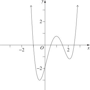
How many stationary points does the graph of \(y=f\left(e^x\right)\) have?
The diagram shows the graph of \(y=f^{\prime}(x)\).
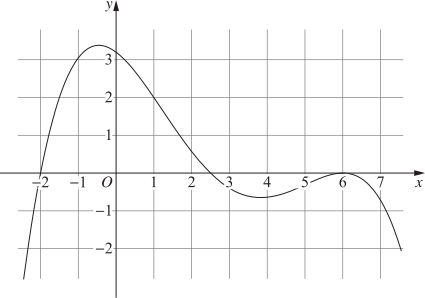
Given \(f(1)=6\), which interval includes the best estimate for \(f(1.1)\) ?
When \(x=-2\) on the curve \(y=f(x)\), the following is true:
\(\dfrac{dy}{dx}<0\) and \(\dfrac{d^2 y}{d x^2}>0\)
At \(x=-2, f(x)\) is
Given \(y=x e^{-3 x}\), prove that
\(\dfrac{d^2 y}{d x^2}+6 \dfrac{d y}{d x}+9 y=0\) (3 marks)
--- 7 WORK AREA LINES (style=lined) ---
A function is defined as \(f(x)=\dfrac{x-h}{(x+1)(x-4)}\)
Determine the range of \(h\) where the graph of \(f(x)\) have no turning points. (3 marks)
--- 9 WORK AREA LINES (style=lined) ---
The function \(f(x)=\dfrac{x}{2}+\dfrac{2}{x}\) undergoes the following sequence of transformations to become \(g(x)\):
The function \(g\) has a local minimum at the point with the coordinates
The graph of the function \(f(x) = \ln(1 + x^{2})\) is shown.
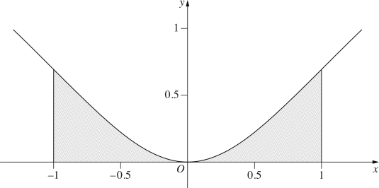
--- 10 WORK AREA LINES (style=lined) ---
\begin{array} {|c|c|c|c|c|c|}
\hline
\rule{0pt}{2.5ex} x \rule[-1ex]{0pt}{0pt} & 0 & 0.25 & 0.5 & 0.75 & 1 \\
\hline
\rule{0pt}{2.5ex} \ln(1+x^2) \rule[-1ex]{0pt}{0pt} & \ \ \ \ 0\ \ \ \ & 0.0606 & 0.2231 & 0.4463 & 0.6931 \\
\hline
\end{array}
--- 5 WORK AREA LINES (style=lined) ---
--- 5 WORK AREA LINES (style=lined) ---
The graph of the function \(g(x)\) is shown.
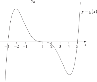
Using the graph, complete the table with the words positive, zero or negative as appropriate. (3 marks)
--- 0 WORK AREA LINES (style=lined) ---
\begin{array} {|l|c|}
\hline
\rule{0pt}{2.5ex} \textit{\(x\)-value} \rule[-1ex]{0pt}{0pt} & \textit{First derivative of \(g(x)\) at \(x\)} \rule[-1ex]{0pt}{0pt} & \textit{Second derivative of \(g(x)\) at \(x\)} \\
\hline
\rule{0pt}{2.5ex} \text{\(x=-3\)} \rule[-1ex]{0pt}{0pt} & \text{ } \rule[-1ex]{0pt}{0pt} & \text{ } \\
\hline
\rule{0pt}{2.5ex} \text{\(x=1\)} \rule[-1ex]{0pt}{0pt} & \text{ } \rule[-1ex]{0pt}{0pt} & \text{ } \\
\hline
\rule{0pt}{2.5ex} \text{\(x=5\)} \rule[-1ex]{0pt}{0pt} & \text{ } \rule[-1ex]{0pt}{0pt} & \text{ } \\
\hline
\end{array}
The graph of \(f(x)\) is drawn below. Draw a sketch of \(f^{\prime}(x)\) on the same graph. (2 marks)
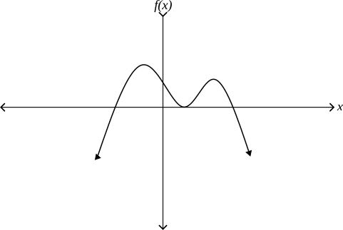
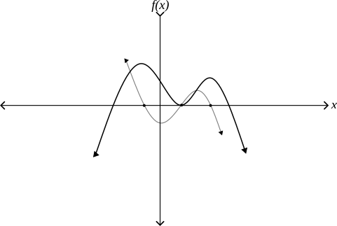
\(\text{Plot x-intercepts at the x-values of turning points.}\)
\(\text{Determine if gradient of}\ f(x)\ \text{is positive/negative to draw shape.}\)
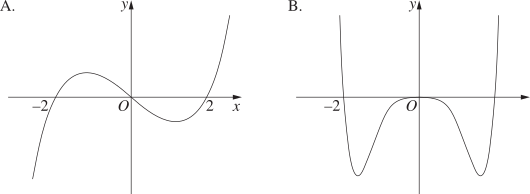
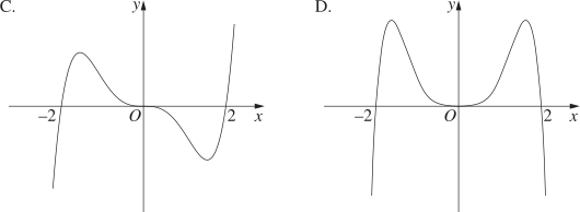
The following table gives the signs of the first and second derivatives of a function \(y=f(x)\) for different values of \(x\).
| \(x\) | \(-2\ \ \) | \(\ 0\ \) | \(\ 2\ \) |
| \( f^{\prime}(x) \) | \(+\) | \(0\) | \(+\) |
| \(f^{\prime\prime}(x)\) | \(-\) | \(0\) | \(+\) |
Which of the following is a possible sketch of \(y=f(x)\)?
For what values of `x` is `f(x) = x^2-2x^3` increasing? (3 marks)
--- 5 WORK AREA LINES (style=lined) ---
The diagram shows part of `y = f(x)` which has a local minimum at `x =-2` and a local maximum at `x = 3`.
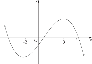
Which of the following shows the correct relationship between `f^(primeprime)(-2), \ f(0)` and `f^(prime)(3)`?
The graph shows two functions `y = f(x)` and `y = g(x)`.
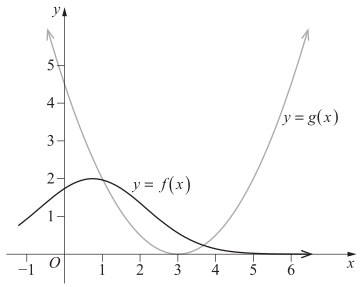
Define `h(x) = f(g(x))`.
How many stationary points does `y = h(x)` have for `1 <= x <= 5`?
Which of the following could represent the graph of `y = −x^2 + bx + 1`, where `b > 0`?
| A. | 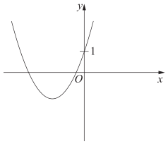 |
B. | 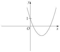 |
| C. | 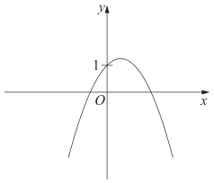 |
D. | 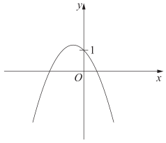 |
Let `f(x) = x^3 + kx^2 + 3x-5`, where `k` is a constant.
Find the values of `k` for which `f(x)` has NO stationary points. (3 marks)
--- 6 WORK AREA LINES (style=lined) ---
`f(x) = x^3 + kx^2 + 3x-5`♦ Mean mark 49%.
`f^{prime}(x) = 3x^2 + 2kx + 3`
`text(No S.P.’s exist if)\ f^{prime}(x)\ text(has no roots,)`
| `Delta` | `< 0` |
| `b^2-4ac` | `< 0` |
| `(2k)^2-4 xx 3 xx 3` | `< 0` |
| `4k^2-36` | `< 0` |
| `k^2-9` | `< 0` |
| `(k-3) (k + 3)` | `< 0` |
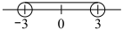
`:. -3 < k < 3`
The diagram shows the graph of `f^{prime}(x)`, the derivative of a function.
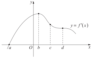
For what value of `x` does the graph of the function `f(x)` have a point of inflection?
The function `f(x)` is defined for `a <= x <= b.`
On this interval, `f ^{prime}(x) > 0 and f^{prime prime}(x) < 0.`
Which graph best represents `y = f(x)`?
| (A) | 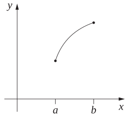 |
(B) | 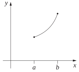 |
| (C) | 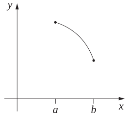 |
(D) | 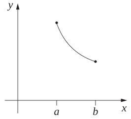 |
The diagram shows the graph of a function `f(x)`.
The graph has a horizontal point of inflection at `A`, a point of inflection at `B` and a maximum turning point at `C`.

On the diagram above, sketch the graph of the derivative `f^{prime}(x)`. (3 marks)
--- 0 WORK AREA LINES (style=lined) ---

Find the coordinates of the stationary point on the graph `y = e^x-ex`, and determine its nature. (3 marks)
--- 6 WORK AREA LINES (style=lined) ---

The diagram shows the graph of a function `y = f(x)`.
--- 1 WORK AREA LINES (style=lined) ---
--- 2 WORK AREA LINES (style=lined) ---
--- 7 WORK AREA LINES (style=blank) ---
a. `f^{prime}(x) < 0\ text(when)`
`-1 < x < 3`
b. `text(As)\ x -> oo`
`f^{prime}(x) -> 0`
c.

a. `f^{prime}(x) < 0\ text(when)`
`-1 < x < 3`
b. `text(As)\ x -> oo,`
`f^{prime}(x) -> 0`
c.
Let `y=f(x)` be a function defined for `0 <= x <= 6`, with `f(0)=0`.
The diagram shows the graph of the derivative of `f`, `y = f^{prime}(x)`.

The shaded region `A_1` has area 4 square units. The shaded region `A_2` has area 4 square units.
--- 2 WORK AREA LINES (style=lined) ---
--- 3 WORK AREA LINES (style=lined) ---
--- 3 WORK AREA LINES (style=lined) ---
--- 8 WORK AREA LINES (style=lined) ---
a. `f(x)\ text(is increasing when)\ 0 <= x < 2`
b. `text(MAX value of)\ f(x) = 4`
c. `-6`
d.
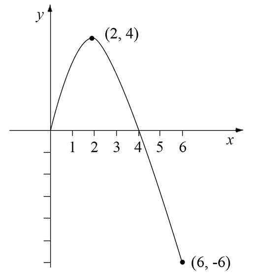
| a. | `f(x)\ text(is increasing when)\ \ f^{prime}(x) > 0` |
| `text(From the graph)` | |
| `f(x)\ text(is increasing when)\ 0 <= x < 2` |
| b. | `f^{prime}(x) = 0\ \ text(when)\ \ x=2` |
| `:.\ text(MAX at)\ \ x = 2` | |
| `int_0^2 f^{prime}(x)\ dx = 4\ \ \ (text(given since)\ A_1 = 4 text{)}` | |
| `text(We also know)` |
| `int_0^2\ f^{prime}(x)\ dx` | `= [f(x)]_0^2` |
| `= f(2)-f(0)` | |
| `= f(2)\ \ \ \ text{(since}\ f(0) = 0 text{)}` |
`=> f(2) = 4`
`:.\ text(MAX value of)\ \ f(x) = 4`
| c. | `int_0^4 f^{prime}(x)` | `= A_1-A_2` |
| `=0` |
`text(We also know)`
| `int_0^4 f^{prime}(x)\ dx` | `= int_2^4 f^{prime}(x)\ dx + int_0^2 f^{prime}(x)\ dx` |
| `=[f(x)]_2^4 + 4` | |
| `= f(4)-f(2) + 4\ \ \ (text(note)\ f(2)=4)` | |
| `=f(4)` |
`=> f(4) = 0`
`text(Gradient)=-3\ text(from)\ \ x = 4\ \ text(to)\ \ x = 6`
| `:.\ f(6)` | `=-3 (6- 4)` |
| `=-6` |
| d. | |
Let `f(x) = x^3-3x^2 + kx + 8`, where `k` is a constant.
Find the values of `k` for which `f(x)` is an increasing function. (2 marks)
--- 5 WORK AREA LINES (style=lined) ---
The graph `y = f(x)` in the diagram has a stationary point when `x = 1`, a point of inflection when `x = 3`, and a horizontal asymptote `y =-2`.

Sketch the graph `y = f^{prime}(x)` , clearly indicating its features at `x = 1` and at `x = 3`, and the shape of the graph as `x -> oo`. (3 marks)
--- 5 WORK AREA LINES (style=blank) ---

The diagram shows the graph `f(x)`.

Which of the following statements is true?
The cubic `y = ax^3 + bx^2 + cx + d` has a point of inflection at `x = p`.
Show that `p=-b/(3a)`. (2 marks)
--- 5 WORK AREA LINES (style=lined) ---
The diagram shows points `A`, `B`, `C` and `D` on the graph `y = f(x)`.

At which point is `f^{prime}(x) > 0` and ` f^{primeprime}(x)= 0`?