Draw the symbols which match the electronic components named in the table. (3 marks) --- 0 WORK AREA LINES (style=lined) ---

Show Answers Only
 Show Worked Solution
Mean mark 57%.
Show Worked Solution
Mean mark 57%.
CHEMISTRY, M8 2023 HSC 26
Nitric acid can be produced industrially using the process shown.

- A mixture of \( \ce{NO2} \) and \( \ce{N2O4} \) enters Reactor 3 , where only \(\ce{NO}_2\) is consumed by the reaction with water.
- Explain, with respect to Le Chatelier's principle, what happens to the \( \ce{N2O4} \). (2 marks)
--- 6 WORK AREA LINES (style=lined) ---
- Explain TWO improvements that can be made to the design of the process shown. (3 marks)
--- 8 WORK AREA LINES (style=lined) ---
BIOLOGY, M5 2022 HSC 31b
Lung cancer can be linked to genetic causes. One of the genes frequently studied in lung cancer tissue is the Epidermal Growth Factor Receptor (EGFR) gene. It codes for EGFR protein, which is composed of one polypeptide chain.
- Construct a flow chart to outline the synthesis of the EGFR protein from the EGFR gene. (4 marks)
--- 12 WORK AREA LINES (style=blank) ---
The structure of the EGFR protein includes a receptor and an enzyme component. The function of the protein is to help the cell to regulate cell division.
EGFR mutations are present in about 32% of cases of Non-Small Cell Lung Cancer (the most common type of lung cancer).
- Explain how a mutation in the EGFR gene could result in changes in protein structure and function to increase the risk of lung cancer. (4 marks)
--- 8 WORK AREA LINES (style=lined) ---
Show Answers Only
i.

ii. Explanation
- A mutation is a permanent change to any section of DNA.
- It can include the change in a single nucleotide base, the deletion or insertion of a base, which will alter all codons proceeding it, or the translation, deletion or addition or entire segments of a chromosome.
- If this occurred in the EGFR gene, this will be copied onto the mRNA, which will be transcribed into the EGFR protein.
- The change of the removal or addition of certain amino acids within the polypeptide chain or even the change in a single amino acid will change the function of the protein or make it unusable at all. In rare cases, this could be beneficial, or a change in an amino acid will be insignificant and not change the proteins shape.
- In most cases however, the mutation on the EFGR gene will render it useless, leading to uncontrolled cell division (cancer).
Show Worked Solution
i.
♦♦♦ Mean mark (i) 28%.
ii. Explanation
- A mutation is a permanent change to any section of DNA.
- It can include the change in a single nucleotide base, the deletion or insertion of a base, which will alter all codons proceeding it, or the translation, deletion or addition or entire segments of a chromosome.
- If this occurred in the EGFR gene, this will be copied onto the mRNA, which will be transcribed into the EGFR protein.
- The change of the removal or addition of certain amino acids within the polypeptide chain or even the change in a single amino acid will change the function of the protein or make it unusable at all. In rare cases, this could be beneficial, or a change in an amino acid will be insignificant and not change the proteins shape.
- In most cases however, the mutation on the EFGR gene will render it useless, leading to uncontrolled cell division (cancer).
♦♦ Mean mark (ii) 32%.
CHEMISTRY, M7 2020 HSC 29
| The flow chart shows reactions involving five different organic compounds, | to |

| Draw the structure of each compound | to | in the corresponding space provided. (5 marks) |


--- 0 WORK AREA LINES (style=lined) ---
Show Answers Only


Show Worked Solution
CHEMISTRY, M7 2022 HSC 9 MC
What is the structure of `\text{CH}_3\text{C}(\text{CH}_3)_2\text{CH}_2\text{CH}(\text{CH}_3)_2`?


PHYSICS, M6 2019 HSC 7 MC
A bar magnet is moved away from a stationary coil.
Which diagram correctly shows the direction of the induced current in the coil and the resulting magnetic polarity of the coil?


MATRICES, FUR2 2020 VCAA 1
The three major shopping centres in a large city, Eastmall `(E)`, Grandmall `(G)` and Westmall `(W)`, are owned by the same company.
The total number of shoppers at each of the centres at 1.00 pm on a typical day is shown in matrix `V`.
`qquad qquad qquad {:(qquad qquad qquad \ E qquad qquad G qquad qquad \ W),(V = [(2300,2700,2200)]):}`
- Write down the order of matrix `V`. (1 mark)
Each of these centres has three major shopping areas: food `(F)`, clothing `(C)` and merchandise `(M)`.
The proportion of shoppers in each of these three areas at 1.00 pm on a typical day is the same at all three centres and is given in matrix `P` below
`qquad qquad qquad P = [(0.48), (0.27), (0.25)] {:(F),(C),(M):}
- Grandmall’s management would like to see 700 shoppers in its merchandise area at 1.00 pm.
If this were to happen, how many shoppers, in total, would be at Grandmall at this time? (1 mark)
- The matrix `Q = P xx V` is shown below. Two of the elements of this matrix are missing.
`{:(quad qquad qquad qquad \ E qquad qquad G qquad qquad W), (Q = [(1104, \ text{___}, 1056 ), (621,\ text{___}, 594), (575, 675, 550)]{:(F),(C), (M):}):}`
-
- Complete matrix `Q` above by filling in the missing elements. (1 mark)
--- 0 WORK AREA LINES (style=lined) ---
- The element in row `i` and column `j` of matrix `Q` is `q_(ij)`.
- What does the element `q_23` represent? (1 mark)
--- 2 WORK AREA LINES (style=lined) ---
- Complete matrix `Q` above by filling in the missing elements. (1 mark)
The average daily amount spent, in dollars, by each shopper in each of the three areas at Grandmall in 2019 is shown in matrix `A_2019` below.
`qquad qquad A_2019 = [(21.30), (34.00), (14.70)] {:(F),(C),(M):}`
On one particular day, 135 shoppers spent the average daily amount on food, 143 shoppers spent the average daily amount on clothing and 131 shoppers spent the average daily amount on merchandise.
- Write a matrix calculation, using matrix `A_2019`, showing that the total amount spent by all these shoppers is $9663.20 (1 mark)
--- 3 WORK AREA LINES (style=lined) ---
- In 2020, the average daily amount spent by each shopper was expected to change by the percentage shown in the table below.
Area food clothing merchandise Expected change increase by 5% decrease by 15% decrease by 1% The average daily amount, in dollars, expected to be spent in each area in 2020 can be determined by forming the matrix product
- `qquad qquad A_2020 = K xx A_2019`
- Write down matrix `K`. (1 mark)
--- 3 WORK AREA LINES (style=lined) ---
CORE, FUR2 2020 VCAA 6
The table below shows the mean age, in years, and the mean height, in centimetres, of 648 women from seven different age groups.

- What was the difference, in centimetres, between the mean height of the women in their twenties and the mean height of the women in their eighties? (1 mark)
--- 1 WORK AREA LINES (style=lined) ---
A scatterplot displaying this data shows an association between the mean height and the mean age of these women. In an initial analysis of the data, a line is fitted to the data by eye, as shown.

- Describe this association in terms of strength and direction. (1 mark)
--- 1 WORK AREA LINES (style=lined) ---
- The line on the scatterplot passes through the points (20,168) and (85,157).
Using these two points, determine the equation of this line. Write the values of the intercept and the slope in the appropriate boxes below.
Round your answers to three significant figures. (1 mark)
--- 0 WORK AREA LINES (style=lined) ---
| mean height = |
|
+ |
|
× mean age |
- In a further analysis of the data, a least squares line was fitted.
The associated residual plot that was generated is shown below.

The residual plot indicates that the association between the mean height and the mean age of women is non-linear.
The data presented in the table in part a is repeated below. It can be linearised by applying an appropriate transformation to the variable mean age.

Apply an appropriate transformation to the variable mean age to linearise the data. Fit a least squares line to the transformed data and write its equation below.
Round the values of the intercept and the slope to four significant figures. (2 marks)
--- 5 WORK AREA LINES (style=lined) ---

NETWORKS, FUR2-NHT 2019 VCAA 3
The zoo’s management requests quotes for parts of the new building works.
Four businesses each submit quotes for four different tasks.
Each business will be offered only one task.
The quoted cost, in $100 000, of providing the work is shown in Table 1 below.

The zoo’s management wants to complete the new building works at minimum cost.
The Hungarian algorithm is used to determine the allocation of tasks to businesses.
The first step of the Hungarian algorithm involves row reduction; that is, subtracting the smallest element in each row of Table 1 from each of the elements in that row.
The result of the first step is shown in Table 2 below.

The second step of the Hungarian algorithm involves column reduction; that is, subtracting the smallest element in each column of Table 2 from each of the elements in that column.
The results of the second step of the Hungarian algorithm are shown in Table 3 below. The values of Task 1 are given as `A, B, C` and `D`.

- Write down the values of `A, B, C` and `D`. (1 mark)
--- 1 WORK AREA LINES (style=lined) ---
- The next step of the Hungarian algorithm involves covering all the zero elements with horizontal or vertical lines. The minimum number of lines required to cover the zeros is three.
Draw these three lines on Table 3 above. (1 mark)
--- 0 WORK AREA LINES (style=lined) ---
- An allocation for minimum cost is not yet possible.
When all steps of the Hungarian algorithm are complete, a bipartite graph can show the allocation for minimum cost.
Complete the bipartite graph below to show this allocation for minimum cost. (1 mark)
--- 4 WORK AREA LINES (style=lined) ---

- Business 4 has changed its quote for the construction of the pathways. The new cost is $1 000 000. The overall minimum cost of the building works is now reduced by reallocating the tasks.
How much is this reduction? (1 mark)
--- 6 WORK AREA LINES (style=lined) ---
Show Worked Solution
a. `A = 2, \ B = 1, \ C = 1, \ D = 0`
| b. |  |
c. `text(After next step:)`

`text(Allocation): `

d. `text{Hungarian Algorithm table (complete):}`

`text(Allocation): B2 -> T3,\ B1 -> T4,\ B3 -> T2,\ B4 -> T1`
`text(C)text(ost) = 4 + 7 + 8 + 10 = 29`
`text(Previous cost) = 5 + 10 + 8 + 8 = 31`
| `:.\ text(Reduction)` | `= 2 xx 100\ 000` |
| `= $200\ 000` |
Data Analysis, GEN2 2019 NHT 5
A random sample of 12 mammals drawn from a population of 62 types of mammals was categorized according to two variables. likelihood of attack (1 = low, 2 = medium, 3 = high) exposure to attack during sleep (1 = low, 2 = medium, 3 = high) The data is shown in the following table. --- 0 WORK AREA LINES (style=lined) --- The following two-way frequency table was formed from the data generated when the entire population of 62 types of mammals was similarly categorized. --- 5 WORK AREA LINES (style=lined) --- --- 2 WORK AREA LINES (style=lined) --- --- 4 WORK AREA LINES (style=lined) ---


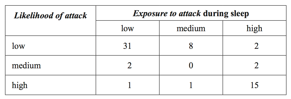
Show Answers Only

`= 50 %`
`text(of attack is associated with low exposure to attack during sleep.)`
`text(- 91%) \ ({31}/{34}) \ text(of animals with low exposure to attack)`
`text(during sleep, have a low likelihood of attack.)`
`text(- Similarly, 89% of animals with a medium exposure to attack during)`
`text(sleep have a low likelihood of attack.)`
`text(- 11% of animals with a high exposure to attack during sleep have)`
`text(a low likelihood of attack)`
a. b. i. `15` iii. `text(The data supports the contention that animals with a low likelihood)` `text(of attack is associated with low exposure to attack during sleep.)` `text(- 91%) \ ({31}/{34}) \ text(of animals with low exposure to attack)` `text(during sleep, have a low likelihood of attack.)` `text(- Similarly, 89% of animals with a medium exposure to attack during)` `text(sleep have a low likelihood of attack.)` `text(- 11% of animals with a high exposure to attack during sleep have)` `text(a low likelihood of attack)`Show Worked Solution
ii. `text(Percentage)`
`= (2)/(4) xx 100`
`= 50%`
Data Analysis, GEN2 2019 NHT 3
The life span, in years, and gestation period, in days, for 19 types of mammals are displayed in the table below.

- A least squares line that enables life span to be predicted from gestation period is fitted to this data.
- Name the explanatory variable in the equation of this least squares line. (1 mark)
--- 1 WORK AREA LINES (style=lined) ---
- Determine the equation of the least squares line in terms of the variables life span and gestation period.
- Round the numbers representing the intercept and slope to three significant figures. (2 marks)
--- 2 WORK AREA LINES (style=lined) ---
- Write the value of the correlation rounded to three decimal places. (1 mark)
--- 2 WORK AREA LINES (style=lined) ---
Data Analysis, GEN2 2019 NHT 1
The table below displays the average sleep time, in hours, for a sample of 19 types of mammals.

- Which of the two variables, type of mammal or average sleep time, is a nominal variable? (1 mark)
--- 1 WORK AREA LINES (style=lined) ---
- Determine the mean and standard deviation of the variable average sleep time for this sample of mammals.
- Round your answer to one decimal place. (1 mark)
--- 2 WORK AREA LINES (style=lined) ---
- The average sleep time for a human is eight hours.
- What percentage of this sample of mammals has an average sleep time that is less than the average sleep time for a human.
- Round your answer to one decimal place. (1 mark)
--- 2 WORK AREA LINES (style=lined) ---
- The sample is increase in size by adding in the average sleep time of the little brown bat.
- Its average sleep time is 19.9 hours.
- By how many many hours will the range for average sleep time increase when the average sleep time for the little brown bat is added to the sample? (1 mark)
--- 2 WORK AREA LINES (style=lined) ---
GRAPHS, FUR2 2019 VCAA 3
Members of the association will travel to a conference in cars and minibuses:
- Let `x` be the number of cars used for travel.
- Let `y` be the number of minibuses used for travel.
- A maximum of eight cars and minibuses in total can be used.
- At least three cars must be used.
- At least two minibuses must be used.
The constraints above can be represented by the following three inequalities.
`text(Inequality 1) qquad qquad x + y <= 8`
`text(Inequality 2) qquad qquad x >= 3`
`text(Inequality 3) qquad qquad y >= 2`
- Each car can carry a total of five people and each minibus can carry a total of 10 people.
A maximum of 60 people can attend the conference.
Use this information to write Inequality 4. (1 mark)
The graph below shows the four lines representing Inequalities 1 to 4.
Also shown on this graph are four of the integer points that satisfy Inequalities 1 to 4. Each of these integer points is marked with a cross (✖).

- On the graph above, mark clearly, with a circle (o), the remaining integer points that satisfy Inequalities 1 to 4. (1 mark)
Each car will cost $70 to hire and each minibus will cost $100 to hire.
- What is the cost for 60 members to travel to the conference? (1 mark)
- What is the minimum cost for 55 members to travel to the conference? (1 mark)
- Just before the cars were booked, the cost of hiring each car increased.
The cost of hiring each minibus remained $100.
All original constraints apply.
If the increase in the cost of hiring each car is more than `k` dollars, then the maximum cost of transporting members to this conference can only occur when using six cars and two minibuses.
Determine the value of `k`. (1 mark)
Show Worked Solution
a. `5x + 10y <= 60`
| b. |  |
c. `text(Consider the line)\ \ 5x + 10y = 60\ \ text(on the graph)`
`text(Touches the feasible region at)\ (4, 4)\ text(only)`
`:.\ text (C) text(ost of 60 members)`
`= 4 xx 70 + 4 xx 100`
`= $680`
d. `text(Coordinates that allow 55 to travel) \ => \ (5, 3) and (3, 4)`
`text(C) text(ost)\ (5, 3) = 5 xx 70 + 3 xx 100 = $650`
`text(C) text(ost)\ (3, 4) = 3 xx 70 + 4 xx 100 = $610`
`:.\ text(Minimum cost is $610)`
e. `text(Objective function): \ C = ax + 100y`
`text(Max cost occurs at)\ \ (6, 2)\ \ text(when)\ \ a > 100`
`text{(i.e. graphically when the slope of}\ \ C = ax + 100y`
`text(is steeper than)\ \ x + y= 8 text{)}`
| `:. k + 70` | `= 100` |
| `k` | `= 30` |
MATRICES, FUR2 2019 VCAA 2
The theme park has four locations, Air World `(A)`, Food World `(F)`, Ground World `(G)` and Water World `(W)`.
The number of visitors at each of the four locations is counted every hour.
By 10 am on Saturday the park had reached its capacity of 2000 visitors and could take no more visitors.
The park stayed at capacity until the end of the day
The state matrix, `S_0`, below, shows the number of visitors at each location at 10 am on Saturday.
`S_0 = [(600), (600), (400), (400)] {:(A),(F),(G),(W):}`
- What percentage of the park’s visitors were at Water World `(W)` at 10 am on Saturday? (1 mark)
--- 2 WORK AREA LINES (style=lined) ---
Let `S_n` be the state matrix that shows the number of visitors expected at each location `n` hours after 10 am on Saturday.
The number of visitors expected at each location `n` hours after 10 am on Saturday can be determined by the matrix recurrence relation below.
`{:(qquad qquadqquadqquadqquadqquadqquadqquadqquadqquadqquadqquadqquadqquadqquadqquadqquadqquadqquadqquadqquadqquadqquad text( this hour)),(qquadqquadqquadqquadqquadqquadqquadqquadqquadqquadqquadqquadqquadqquadqquadqquadqquadqquadqquad qquad qquad quad A qquad quad F qquad \ G \ quad quad W),({:S_0 = [(600), (600), (400), (400)], qquad S_(n+1) = T xx S_n quad quad qquad text(where):}\ T = [(0.1,0.2,0.1,0.2),(0.3,0.4,0.6,0.3),(0.1,0.2,0.2,0.1),(0.5,0.2,0.1,0.4)]{:(A),(F),(G),(W):}\ text(next hour)):}`
- Complete the state matrix, `S_1`, below to show the number of visitors expected at each location at 11 am on Saturday. (1 mark)
--- 0 WORK AREA LINES (style=lined) ---
`S_1 = [(\ text{______}\ ), (\ text{______}\ ), (300),(\ text{______}\ )]{:(A),(F),(G),(W):}`
- Of the 300 visitors expected at Ground World `(G)` at 11 am, what percentage was at either Air World `(A)` or Food World `(F)` at 10 am? (1 mark)
--- 3 WORK AREA LINES (style=lined) ---
- The proportion of visitors moving from one location to another each hour on Sunday is different from Saturday.
Matrix `V`, below, shows the proportion of visitors moving from one location to another each hour after 10 am on Sunday.
`qquad qquad {:(qquadqquadqquadqquadqquadtext(this hour)),(qquad qquad qquad \ A qquad quad F qquad \ G \ quad quad W),(V = [(0.3,0.4,0.6,0.3),(0.1,0.2,0.1,0.2),(0.1,0.2,0.2,0.1),(0.5,0.2,0.1,0.4)]{:(A),(F),(G),(W):}\ text(next hour)):}`
Matrix `V` is similar to matrix `T` but has the first two rows of matrix `T` interchanged. - The matrix product that will generate matrix `V` from matrix `T` is
- `qquad qquad V = M xx T`
- where matrix `M` is a binary matrix.
- Write down matrix `M`. (1 mark)
--- 4 WORK AREA LINES (style=lined) ---
MATRICES, FUR2 2019 VCAA 1
The car park at a theme park has three areas, `A, B` and `C`.
The number of empty `(E)` and full `(F)` parking spaces in each of the three areas at 1 pm on Friday are shown in matrix `Q` below.
`{:(qquad qquad qquad \ E qquad F),(Q = [(70, 50),(30, 20),(40, 40)]{:(A),(B),(C):}quad text(area)):}`
- What is the order of matrix `Q`? (1 mark)
--- 1 WORK AREA LINES (style=lined) ---
- Write down a calculation to show that 110 parking spaces are full at 1 pm. (1 mark)
--- 2 WORK AREA LINES (style=lined) ---
Drivers must pay a parking fee for each hour of parking.
Matrix `P`, below, shows the hourly fee, in dollars, for a car parked in each of the three areas.
`{:(qquad qquad qquad qquad qquad text{area}), (qquad qquad qquad A qquad quad quad B qquad qquad C), (P = [(1.30, 3.50, 1.80)]):}`
- The total parking fee, in dollars, collected from these 110 parked cars if they were parked for one hour is calculated as follows.
`qquad qquad qquad P xx L = [207.00]`
where matrix `L` is a `3 xx 1` matrix.
Write down matrix `L`. (1 mark)
--- 2 WORK AREA LINES (style=lined) ---
The number of whole hours that each of the 110 cars had been parked was recorded at 1 pm. Matrix `R`, below, shows the number of cars parked for one, two, three or four hours in each of the areas `A, B` and `C`.
`{:(qquadqquadqquadqquadquadtext(area)),(quad qquadqquadquad \ A qquad B qquad C),(R = [(3, 1, 1),(6, 10, 3),(22, 7,10),(19, 2, 26)]{:(1),(2),(3),(4):}\ text(hours)):}`
- Matrix `R^T` is the transpose of matrix `R`.
Complete the matrix `R^T` below. (1 mark)
--- 0 WORK AREA LINES (style=lined) ---
`qquad R^T = [( , , , , , , , , ), ( , , , , , , , , ), ( , , , , , , , , ), ( , , , , , , , , ), ( , , , , , , , , )]`
- Explain what the element in row 3, column 2 of matrix `R^T` represents. (1 mark)
--- 2 WORK AREA LINES (style=lined) ---
CORE, FUR2 2019 VCAA 5
The scatterplot below shows the atmospheric pressure, in hectopascals (hPa), at 3 pm (pressure 3 pm) plotted against the atmospheric pressure, in hectopascals, at 9 am (pressure 9 am) for 23 days in November 2017 at a particular weather station.

A least squares line has been fitted to the scatterplot as shown.
The equation of this line is
pressure 3 pm = 111.4 + 0.8894 × pressure 9 am
- Interpret the slope of this least squares line in terms of the atmospheric pressure at this weather station at 9 am and at 3 pm. (1 mark)
--- 2 WORK AREA LINES (style=lined) ---
- Use the equation of the least squares line to predict the atmospheric pressure at 3 pm when the atmospheric pressure at 9 am is 1025 hPa.
- Round your answer to the nearest whole number. (1 mark)
--- 2 WORK AREA LINES (style=lined) ---
- Is the prediction made in part b. an example of extrapolation or interpolation? (1 mark)
--- 1 WORK AREA LINES (style=lined) ---
- Determine the residual when the atmospheric pressure at 9 am is 1013 hPa.
- Round your answer to the nearest whole number. (1 mark)
--- 3 WORK AREA LINES (style=lined) ---
- The mean and the standard deviation of pressure 9 am and pressure 3 pm for these 23 days are shown in Table 4 below.

-
- Use the equation of the least squares line and the information in Table 4 to show that the correlation coefficient for this data, rounded to three decimal places, is `r` = 0.966 (1 mark)
--- 3 WORK AREA LINES (style=lined) ---
- What percentage of the variation in pressure 3 pm is explained by the variation in pressure 9 am?
- Round your answer to one decimal place. (1 mark)
--- 2 WORK AREA LINES (style=lined) ---
- Use the equation of the least squares line and the information in Table 4 to show that the correlation coefficient for this data, rounded to three decimal places, is `r` = 0.966 (1 mark)
- The residual plot associated with the least squares line is shown below.

-
- The residual plot above can be used to test one of the assumptions about the nature of the association between the atmospheric pressure at 3 pm and the atmospheric pressure at 9 am.
- What is this assumption? (1 mark)
--- 2 WORK AREA LINES (style=lined) ---
- The residual plot above does not support this assumption.
- Explain why. (1 mark)
--- 2 WORK AREA LINES (style=lined) ---
EXT1 S1 Probability Tables: Negative
Probability Table for Standard Normal Distribution
Negative z-scores
| z | 0.00 | 0.01 | 0.02 | 0.03 | 0.04 | 0.05 | 0.06 | 0.07 | 0.08 | 0.09 |
| -3.4 | 0.0003 | 0.0003 | 0.0003 | 0.0003 | 0.0003 | 0.0003 | 0.0003 | 0.0003 | 0.0003 | 0.0002 |
| -3.3 | 0.0005 | 0.0005 | 0.0005 | 0.0004 | 0.0004 | 0.0004 | 0.0004 | 0.0004 | 0.0004 | 0.0003 |
| -3.2 | 0.0007 | 0.0007 | 0.0006 | 0.0006 | 0.0006 | 0.0006 | 0.0006 | 0.0005 | 0.0005 | 0.0005 |
| -3.1 | 0.0010 | 0.0009 | 0.0009 | 0.0009 | 0.0008 | 0.0008 | 0.0008 | 0.0008 | 0.0007 | 0.0007 |
| -3.0 | 0.0013 | 0.0013 | 0.0013 | 0.0012 | 0.0012 | 0.0011 | 0.0011 | 0.0011 | 0.0010 | 0.0010 |
| -2.9 | 0.0019 | 0.0018 | 0.0018 | 0.0017 | 0.0016 | 0.0016 | 0.0015 | 0.0015 | 0.0014 | 0.0014 |
| -2.8 | 0.0026 | 0.0025 | 0.0024 | 0.0023 | 0.0023 | 0.0022 | 0.0021 | 0.0021 | 0.0020 | 0.0019 |
| -2.7 | 0.0035 | 0.0034 | 0.0033 | 0.0032 | 0.0031 | 0.0030 | 0.0029 | 0.0028 | 0.0027 | 0.0026 |
| -2.6 | 0.0047 | 0.0045 | 0.0044 | 0.0043 | 0.0041 | 0.0040 | 0.0039 | 0.0038 | 0.0037 | 0.0036 |
| -2.5 | 0.0062 | 0.0060 | 0.0059 | 0.0057 | 0.0055 | 0.0054 | 0.0052 | 0.0051 | 0.0049 | 0.0048 |
| -2.4 | 0.0082 | 0.0080 | 0.0078 | 0.0075 | 0.0073 | 0.0071 | 0.0069 | 0.0068 | 0.0066 | 0.0064 |
| -2.3 | 0.0107 | 0.0104 | 0.0102 | 0.0099 | 0.0096 | 0.0094 | 0.0091 | 0.0089 | 0.0087 | 0.0084 |
| -2.2 | 0.0139 | 0.0136 | 0.0132 | 0.0129 | 0.0125 | 0.0122 | 0.0119 | 0.0116 | 0.0113 | 0.0110 |
| -2.1 | 0.0179 | 0.0174 | 0.0170 | 0.0166 | 0.0162 | 0.0158 | 0.0154 | 0.0150 | 0.0146 | 0.0143 |
| -2.0 | 0.0228 | 0.0222 | 0.0217 | 0.0212 | 0.0207 | 0.0202 | 0.0197 | 0.0192 | 0.0188 | 0.0183 |
| -1.9 | 0.0287 | 0.0281 | 0.0274 | 0.0268 | 0.0262 | 0.0256 | 0.0250 | 0.0244 | 0.0239 | 0.0233 |
| -1.8 | 0.0359 | 0.0351 | 0.0344 | 0.0336 | 0.0329 | 0.0322 | 0.0314 | 0.0307 | 0.0301 | 0.0294 |
| -1.7 | 0.0446 | 0.0436 | 0.0427 | 0.0418 | 0.0409 | 0.0401 | 0.0392 | 0.0384 | 0.0375 | 0.0367 |
| -1.6 | 0.0548 | 0.0537 | 0.0526 | 0.0516 | 0.0505 | 0.0495 | 0.0485 | 0.0475 | 0.0465 | 0.0455 |
| -1.5 | 0.0668 | 0.0655 | 0.0643 | 0.0630 | 0.0618 | 0.0606 | 0.0594 | 0.0582 | 0.0571 | 0.0559 |
| -1.4 | 0.0808 | 0.0793 | 0.0778 | 0.0764 | 0.0749 | 0.0735 | 0.0721 | 0.0708 | 0.0694 | 0.0681 |
| -1.3 | 0.0968 | 0.0951 | 0.0934 | 0.0918 | 0.0901 | 0.0885 | 0.0869 | 0.0853 | 0.0838 | 0.0823 |
| -1.2 | 0.1151 | 0.1131 | 0.1112 | 0.1093 | 0.1075 | 0.1056 | 0.1038 | 0.1020 | 0.1003 | 0.0985 |
| -1.1 | 0.1357 | 0.1335 | 0.1314 | 0.1292 | 0.1271 | 0.1251 | 0.1230 | 0.1210 | 0.1190 | 0.1170 |
| -1.0 | 0.1587 | 0.1562 | 0.1539 | 0.1515 | 0.1492 | 0.1469 | 0.1446 | 0.1423 | 0.1401 | 0.1379 |
| -0.9 | 0.1841 | 0.1814 | 0.1788 | 0.1762 | 0.1736 | 0.1711 | 0.1685 | 0.1660 | 0.1635 | 0.1611 |
| -0.8 | 0.2119 | 0.2090 | 0.2061 | 0.2033 | 0.2005 | 0.1977 | 0.1949 | 0.1922 | 0.1894 | 0.1867 |
| -0.7 | 0.2420 | 0.2389 | 0.2358 | 0.2327 | 0.2296 | 0.2266 | 0.2236 | 0.2206 | 0.2177 | 0.2148 |
| -0.6 | 0.2743 | 0.2709 | 0.2676 | 0.2643 | 0.2611 | 0.2578 | 0.2546 | 0.2514 | 0.2483 | 0.2451 |
| -0.5 | 0.3085 | 0.3050 | 0.3015 | 0.2981 | 0.2946 | 0.2912 | 0.2877 | 0.2843 | 0.2810 | 0.2776 |
| -0.4 | 0.3446 | 0.3409 | 0.3372 | 0.3336 | 0.3300 | 0.3264 | 0.3228 | 0.3192 | 0.3156 | 0.3121 |
| -0.3 | 0.3821 | 0.3783 | 0.3745 | 0.3707 | 0.3669 | 0.3632 | 0.3594 | 0.3557 | 0.3520 | 0.3483 |
| -0.2 | 0.4207 | 0.4168 | 0.4129 | 0.4090 | 0.4052 | 0.4013 | 0.3974 | 0.3936 | 0.3897 | 0.3859 |
| -0.1 | 0.4602 | 0.4562 | 0.4522 | 0.4483 | 0.4443 | 0.4404 | 0.4364 | 0.4325 | 0.4286 | 0.4247 |
| 0.0 | 0.5000 | 0.4960 | 0.4920 | 0.4880 | 0.4840 | 0.4801 | 0.4761 | 0.4721 | 0.4681 | 0.4641 |
EXT1 S1 Probability Tables: Positive v2
Probability Table for Standard Normal Distribution
Positive z-scores
| z | 0.00 | 0.01 | 0.02 | 0.03 | 0.04 | 0.05 | 0.06 | 0.07 | 0.08 | 0.09 |
| 0.0 | 0.5000 | 0.5040 | 0.5080 | 0.5120 | 0.5160 | 0.5199 | 0.5239 | 0.5279 | 0.5319 | 0.5359 |
| 0.1 | 0.5398 | 0.5438 | 0.5478 | 0.5517 | 0.5557 | 0.5596 | 0.5636 | 0.5675 | 0.5714 | 0.5753 |
| 0.2 | 0.5793 | 0.5832 | 0.5871 | 0.5910 | 0.5948 | 0.5987 | 0.6026 | 0.6064 | 0.6103 | 0.6141 |
| 0.3 | 0.6179 | 0.6217 | 0.6255 | 0.6293 | 0.6331 | 0.6368 | 0.6406 | 0.6443 | 0.6480 | 0.6517 |
| 0.4 | 0.6554 | 0.6591 | 0.6628 | 0.6664 | 0.6700 | 0.6736 | 0.6772 | 0.6808 | 0.6844 | 0.6879 |
| 0.5 | 0.6915 | 0.6950 | 0.6985 | 0.7019 | 0.7054 | 0.7088 | 0.7123 | 0.7157 | 0.7190 | 0.7224 |
| 0.6 | 0.7257 | 0.7291 | 0.7324 | 0.7357 | 0.7389 | 0.7422 | 0.7454 | 0.7486 | 0.7517 | 0.7549 |
| 0.7 | 0.7580 | 0.7611 | 0.7642 | 0.7673 | 0.7704 | 0.7734 | 0.7764 | 0.7794 | 0.7823 | 0.7852 |
| 0.8 | 0.7881 | 0.7910 | 0.7939 | 0.7967 | 0.7995 | 0.8023 | 0.8051 | 0.8078 | 0.8106 | 0.8133 |
| 0.9 | 0.8159 | 0.8186 | 0.8212 | 0.8238 | 0.8264 | 0.8289 | 0.8315 | 0.8340 | 0.8365 | 0.8389 |
| 1.0 | 0.8413 | 0.8438 | 0.8461 | 0.8485 | 0.8508 | 0.8531 | 0.8554 | 0.8577 | 0.8599 | 0.8621 |
| 1.1 | 0.8643 | 0.8665 | 0.8686 | 0.8708 | 0.8729 | 0.8749 | 0.8770 | 0.8790 | 0.8810 | 0.8830 |
| 1.2 | 0.8849 | 0.8869 | 0.8888 | 0.8907 | 0.8925 | 0.8944 | 0.8962 | 0.8980 | 0.8997 | 0.9015 |
| 1.3 | 0.9032 | 0.9049 | 0.9066 | 0.9082 | 0.9099 | 0.9115 | 0.9131 | 0.9147 | 0.9162 | 0.9177 |
| 1.4 | 0.9192 | 0.9207 | 0.9222 | 0.9236 | 0.9251 | 0.9265 | 0.9279 | 0.9292 | 0.9306 | 0.9319 |
| 1.5 | 0.9332 | 0.9345 | 0.9357 | 0.9370 | 0.9382 | 0.9394 | 0.9406 | 0.9418 | 0.9429 | 0.9441 |
| 1.6 | 0.9452 | 0.9463 | 0.9474 | 0.9484 | 0.9495 | 0.9505 | 0.9515 | 0.9525 | 0.9535 | 0.9545 |
| 1.7 | 0.9554 | 0.9564 | 0.9573 | 0.9582 | 0.9591 | 0.9599 | 0.9608 | 0.9616 | 0.9625 | 0.9633 |
| 1.8 | 0.9641 | 0.9649 | 0.9656 | 0.9664 | 0.9671 | 0.9678 | 0.9686 | 0.9693 | 0.9699 | 0.9706 |
| 1.9 | 0.9713 | 0.9719 | 0.9726 | 0.9732 | 0.9738 | 0.9744 | 0.9750 | 0.9756 | 0.9761 | 0.9767 |
| 2.0 | 0.9772 | 0.9778 | 0.9783 | 0.9788 | 0.9793 | 0.9798 | 0.9803 | 0.9808 | 0.9812 | 0.9817 |
| 2.1 | 0.9821 | 0.9826 | 0.9830 | 0.9834 | 0.9838 | 0.9842 | 0.9846 | 0.9850 | 0.9854 | 0.9857 |
| 2.2 | 0.9861 | 0.9864 | 0.9868 | 0.9871 | 0.9875 | 0.9878 | 0.9881 | 0.9884 | 0.9887 | 0.9890 |
| 2.3 | 0.9893 | 0.9896 | 0.9898 | 0.9901 | 0.9904 | 0.9906 | 0.9909 | 0.9911 | 0.9913 | 0.9916 |
| 2.4 | 0.9918 | 0.9920 | 0.9922 | 0.9925 | 0.9927 | 0.9929 | 0.9931 | 0.9932 | 0.9934 | 0.9936 |
| 2.5 | 0.9938 | 0.9940 | 0.9941 | 0.9943 | 0.9945 | 0.9946 | 0.9948 | 0.9949 | 0.9951 | 0.9952 |
| 2.6 | 0.9953 | 0.9955 | 0.9956 | 0.9957 | 0.9959 | 0.9960 | 0.9961 | 0.9962 | 0.9963 | 0.9964 |
| 2.7 | 0.9965 | 0.9966 | 0.9967 | 0.9968 | 0.9969 | 0.9970 | 0.9971 | 0.9972 | 0.9973 | 0.9974 |
| 2.8 | 0.9974 | 0.9975 | 0.9976 | 0.9977 | 0.9977 | 0.9978 | 0.9979 | 0.9979 | 0.9980 | 0.9981 |
| 2.9 | 0.9981 | 0.9982 | 0.9982 | 0.9983 | 0.9984 | 0.9984 | 0.9985 | 0.9985 | 0.9986 | 0.9986 |
| 3.0 | 0.9987 | 0.9987 | 0.9987 | 0.9988 | 0.9988 | 0.9989 | 0.9989 | 0.9989 | 0.9990 | 0.9990 |
| 3.1 | 0.9990 | 0.9991 | 0.9991 | 0.9991 | 0.9992 | 0.9992 | 0.9992 | 0.9992 | 0.9993 | 0.9993 |
| 3.2 | 0.9993 | 0.9993 | 0.9994 | 0.9994 | 0.9994 | 0.9994 | 0.9994 | 0.9995 | 0.9995 | 0.9995 |
| 3.3 | 0.9995 | 0.9995 | 0.9995 | 0.9996 | 0.9996 | 0.9996 | 0.9996 | 0.9996 | 0.9996 | 0.9997 |
| 3.4 | 0.9997 | 0.9997 | 0.9997 | 0.9997 | 0.9997 | 0.9997 | 0.9997 | 0.9997 | 0.9997 | 0.9998 |
CORE, FUR2 2018 VCAA 3
Table 3 shows the yearly average traffic congestion levels in two cities, Melbourne and Sydney, during the period 2008 to 2016. Also shown is a time series plot of the same data.
The time series plot for Melbourne is incomplete.

- Use the data in Table 3 to complete the time series plot above for Melbourne. (1 mark)
--- 0 WORK AREA LINES (style=lined) ---
- A least squares line is used to model the trend in the time series plot for Sydney. The equation is
`text(congestion level = −2280 + 1.15 × year)`
- i. Draw this least squares line on the time series plot. (1 mark)
--- 0 WORK AREA LINES (style=lined) ---
- ii. Use the equation of the least squares line to determine the average rate of increase in percentage congestion level for the period 2008 to 2016 in Sydney. (1 mark)
--- 2 WORK AREA LINES (style=lined) ---
iii. Use the least squares line to predict when the percentage congestion level in Sydney will be 43%. (1 mark)
--- 3 WORK AREA LINES (style=lined) ---
The yearly average traffic congestion level data for Melbourne is repeated in Table 4 below.

- When a least squares line is used to model the trend in the data for Melbourne, the intercept of this line is approximately –1514.75556
- Round this value to four significant figures. (1 mark)
--- 1 WORK AREA LINES (style=lined) ---
- Use the data in Table 4 to determine the equation of the least squares line that can be used to model the trend in the data for Melbourne. The variable year is the explanatory variable.
- Write the values of the intercept and the slope of this least squares line in the appropriate boxes provided below.
- Round both values to four significant figures. (2 marks)
--- 0 WORK AREA LINES (style=lined) ---
| congestion level = |
|
+ |
|
× year |
- Since 2008, the equations of the least squares lines for Sydney and Melbourne have predicted that future traffic congestion levels in Sydney will always exceed future traffic congestion levels in Melbourne.
Explain why, quoting the values of appropriate statistics. (2 marks)
--- 5 WORK AREA LINES (style=lined) ---
Show Worked Solution
| a. |  |
| b.i. |  |
b.ii. `text(The least squares line is 1.15% higher each year.)`♦ Mean mark (b)(ii) 36%.
COMMENT: Major problems caused by part (b)(ii). Review!
` :.\ text(Average rate of increase) = 1.15 text(%)`
| b.iii. | `text(Find year when:)` | |
| `43` | `= -2280 + 1.15 xx text(year)` | |
| `text(year)` | `= 2323/1.15` | |
| `= 2020` | ||
c. `-1515`
d. `text(congestion level) = -1515 + 0.7667 xx text(year)`
e. `text(Melbourne congestion level in 2008)`♦♦♦ Mean mark 18%.
`= -1515 + 0.7667 xx 2008`
`= 24.5 text(%)`
`text{In 2008 Sydney has higher congestion (29.2 > 24.5)}`
`text(After 2008, Sydney congestion grows at 1.15% per)`
`text(year and Melbourne grows at 0.7667% per year.)`
`:.\ text(Sydney predicted to always exceed Melbourne.)`
CORE, FUR2 2018 VCAA 1
The data in Table 1 relates to the impact of traffic congestion in 2016 on travel times in 23 cities in the United Kingdom (UK). The four variables in this data set are: --- 1 WORK AREA LINES (style=lined) --- --- 1 WORK AREA LINES (style=lined) --- --- 1 WORK AREA LINES (style=lined) --- --- 0 WORK AREA LINES (style=lined) --- --- 3 WORK AREA LINES (style=lined) --- Traffic congestion can lead to an increase in travel times in cities. The dot plot and boxplot below both show the increase in travel time due to traffic congestion, in minutes per day, for the 23 UK cities. --- 1 WORK AREA LINES (style=lined) --- --- 3 WORK AREA LINES (style=lined) ---


a. `3\-text(city, congestion level, size)` b. `2\-text(congestion level, size)` c. `text(Newcastle-Sunderland and Liverpool)` g. `IQR = 39-30 = 9` `text(Calculate the Upper Fence:)`Show Worked Solution
d.

e.
`text(Percentage)`
`= text(Number of small cities high congestion)/text(Number of small cities) xx 100`
`= 4/16 xx 100`
`= 25 text(%)`
f. `text(Positively skewed)`
`Q_3 + 1.5 xx IQR`
`= 39 + 1.5 xx 9`
`= 52.5`
Harder Ext1 Topics, EXT2 2018 HSC 13d
The points `P(cp, c/p)` and `Q(cp, c/q)` lie on the rectangular hyperbola `xy = c^2`.
The line `PQ` has equation `x + pqy = c(p + q)`. (Do NOT prove this.)
The `x` and `y` intercepts of `PQ` are `R` and `S` respectively, as shown in the diagram.

- Show that `PS = QR`. (3 marks)
The point `T(2at, at^2)` lies on the parabola `x^2 = 4ay`. The tangent to the parabola at `T` intersects the rectangular hyperbola `xy = c^2` at `A` and `B` and has equation `y = tx - at^2`. (Do NOT prove this.) The point `M` is the midpoint of the interval `AB`. One such case is shown in the diagram.

- Using part (i), or otherwise, show that `M` lies on the parabola `2x^2 = −ay`. (2 marks)
Algebra, MET2 2017 VCAA 4
Let `f : R → R :\ f (x) = 2^(x + 1)-2`. Part of the graph of `f` is shown below.

- The transformation `T: R^2 -> R^2, \ T([(x),(y)]) = [(x),(y)] + [(c),(d)]` maps the graph of `y = 2^x` onto the graph of `f`.
State the values of `c` and `d`. (2 marks)
--- 5 WORK AREA LINES (style=lined) ---
- Find the rule and domain for `f^(-1)`, the inverse function of `f`. (2 marks)
--- 5 WORK AREA LINES (style=lined) ---
- Find the area bounded by the graphs of `f` and `f^(-1)`. (3 marks)
--- 3 WORK AREA LINES (style=lined) ---
- Part of the graphs of `f` and `f^(-1)` are shown below.

Find the gradient of `f` and the gradient of `f^(-1)` at `x = 0`. (2 marks)
--- 2 WORK AREA LINES (style=lined) ---
The functions of `g_k`, where `k ∈ R^+`, are defined with domain `R` such that `g_k(x) = 2e^(kx)-2`.
- Find the value of `k` such that `g_k(x) = f(x)`. (1 mark)
--- 3 WORK AREA LINES (style=lined) ---
- Find the rule for the inverse functions `g_k^(-1)` of `g_k`, where `k ∈ R^+`. (1 mark)
--- 5 WORK AREA LINES (style=lined) ---
- i. Describe the transformation that maps the graph of `g_1` onto the graph of `g_k`. (1 mark)
--- 3 WORK AREA LINES (style=lined) ---
ii. Describe the transformation that maps the graph of `g_1^(-1)` onto the graph of `g_k^(-1)`. (1 mark)
--- 3 WORK AREA LINES (style=lined) ---
- The lines `L_1` and `L_2` are the tangents at the origin to the graphs of `g_k` and `g_k^(-1)` respectively.
- Find the value(s) of `k` for which the angle between `L_1` and `L_2` is 30°. (2 marks)
--- 6 WORK AREA LINES (style=lined) ---
- Let `p` be the value of `k` for which `g_k(x) = g_k^(−1)(x)` has only one solution.
- i. Find `p`. (2 marks)
--- 4 WORK AREA LINES (style=lined) ---
- ii. Let `A(k)` be the area bounded by the graphs of `g_k` and `g_k^(-1)` for all `k > p`.
- State the smallest value of `b` such that `A(k) < b`. (1 mark)
--- 4 WORK AREA LINES (style=lined) ---
Algebra, MET2 2017 VCAA 2
Sammy visits a giant Ferris wheel. Sammy enters a capsule on the Ferris wheel from a platform above the ground. The Ferris wheel is rotating anticlockwise. The capsule is attached to the Ferris wheel at point `P`. The height of `P` above the ground, `h`, is modelled by `h(t) = 65-55cos((pit)/15)`, where `t` is the time in minutes after Sammy enters the capsule and `h` is measured in metres.
Sammy exits the capsule after one complete rotation of the Ferris wheel.

- State the minimum and maximum heights of `P` above the ground. (1 mark)
--- 2 WORK AREA LINES (style=lined) ---
- For how much time is Sammy in the capsule? (1 mark)
--- 2 WORK AREA LINES (style=lined) ---
- Find the rate of change of `h` with respect to `t` and, hence, state the value of `t` at which the rate of change of `h` is at its maximum. (2 marks)
--- 4 WORK AREA LINES (style=lined) ---
As the Ferris wheel rotates, a stationary boat at `B`, on a nearby river, first becomes visible at point `P_1`. `B` is 500 m horizontally from the vertical axis through the centre `C` of the Ferris wheel and angle `CBO = theta`, as shown below.

- Find `theta` in degrees, correct to two decimal places. (1 mark)
--- 3 WORK AREA LINES (style=lined) ---
Part of the path of `P` is given by `y = sqrt(3025-x^2) + 65, x ∈ [-55,55]`, where `x` and `y` are in metres.
- Find `(dy)/(dx)`. (1 mark)
--- 2 WORK AREA LINES (style=lined) ---
As the Ferris wheel continues to rotate, the boat at `B` is no longer visible from the point `P_2(u, v)` onwards. The line through `B` and `P_2` is tangent to the path of `P`, where angle `OBP_2 = alpha`.

- Find the gradient of the line segment `P_2B` in terms of `u` and, hence, find the coordinates of `P_2`, correct to two decimal places. (3 marks)
--- 10 WORK AREA LINES (style=lined) ---
- Find `alpha` in degrees, correct to two decimal places. (1 mark)
--- 4 WORK AREA LINES (style=lined) ---
- Hence or otherwise, find the length of time, to the nearest minute, during which the boat at `B` is visible. (2 marks)
--- 5 WORK AREA LINES (style=lined) ---
Show Worked Solution
| a. | `h_text(min)` | `= 65-55` | `h_text(max)` | `= 65 + 55` |
| `= 10\ text(m)` | `= 120\ text(m)` |
b. `text(Period) = (2pi)/(pi/15) = 30\ text(min)`
c. `h^{prime}(t) = (11pi)/3\ sin(pi/15 t)`♦ Mean mark 50%.
MARKER’S COMMENT: A number of commons errors here – 2 answers given, calc not in radian mode, etc …
`text(Solve)\ h^{primeprime}(t) = 0, t ∈ (0,30)`
| `t = 15/2\ \ text{(max)}` | `text(or)` | `t = 45/2\ \ text{(min – descending)}` |
`:. t = 7.5`
| d. |  |
♦ Mean mark 36%.
MARKER’S COMMENT: Choosing degrees vs radians in the correct context was critical here.
| `tan(theta)` | `= 65/500` |
| `:. theta` | `=7.406…` |
| `= 7.41^@` |
| e. | `(dy)/(dx)` | `= (-x)/(sqrt(3025-x^2))` |
| f. |  |
`P_2(u,sqrt(3025-u^2) + 65),\ \ B(500,0)`
| `:. m_(P_2B)` | `= (sqrt(3025-u^2) + 65)/(u-500)` |
`text{Using part (e), when}\ \ x=u,`♦♦♦ Mean mark part (f) 18%.
MARKER’S COMMENT: Many students were unable to use the rise over run information to calculate the second gradient.
`dy/dx=(-u)/(sqrt(3025-u^2))`
`text{Solve (by CAS):}`
| `(sqrt(3025-u^2) + 65)/(u-500)` | `= (-u)/(sqrt(3025-u^2))\ \ text(for)\ u` |
`u=12.9975…=13.00\ \ text{(2 d.p.)}`
| `:. v` | `= sqrt(3025-(12.9975…)^2) + 65` |
| `= 118.4421…` | |
| `= 118.44\ \ text{(2 d.p.)}` |
`:.P_2(13.00, 118.44)`
♦♦♦ Mean mark part (g) 7%.
| g. | `tan alpha` | `=v/(500-u)` |
| `= (118.442…)/(500-12.9975…)` | ||
| `:. alpha` | `= 13.67^@\ \ text{(2 d.p.)}` |
| h. |  |
♦♦♦ Mean mark 5%.
`text(Find the rotation between)\ P_1 and P_2:`
`text(Rotation to)\ P_1 = 90-7.41=82.59^@`
`text(Rotation to)\ P_2 = 180-13.67=166.33^@`
`text(Rotation)\ \ P_1 → P_2 = 166.33-82.59 = 83.74^@`
| `:.\ text(Time visible)` | `= 83.74/360 xx 30\ text(min)` |
| `=6.978…` | |
| `= 7\ text{min (nearest degree)}` |
MATRICES, FUR1 2017 VCAA 4 MC
A permutation matrix, `P`, can be used to change `[(F),(E),(A),(R),(S)]` into `[(S),(A),(F),(E),(R)]`.
Matrix `P` is
| A. |
`[(0,0,1,0,1),(0,0,1,1,0),(1,1,0,0,0),(0,1,0,0,1),(1,0,0,1,0)]`
|
B. |
`[(0,0,0,1,0),(0,0,1,0,0),(0,1,0,0,0),(0,0,0,0,1),(1,0,0,0,0)]`
|
| C. |
`[(0,0,0,0,1),(0,0,1,0,0),(1,0,0,0,0),(0,1,0,0,0),(0,0,0,1,0)]`
|
D. |
`[(1,0,0,0,1),(0,1,1,0,0),(1,0,1,0,0),(0,1,0,1,0),(0,0,0,1,1)]`
|
| E. |
`[(0,0,0,0,1),(0,0,1,0,0),(0,1,0,0,0),(1,0,0,0,0),(0,0,0,1,0)]`
|
GRAPHS, FUR1 2017 VCAA 8 MC
The shaded area in the graph below shows the feasible region for a linear programming problem.

The objective function is given by
`Z = mx + ny`
Which one of the following statements is not true?
- When `m = 4` and `n = 1`, the minimum value of `Z` is at point `A`.
- When `m = 1` and `n = 6`, the maximum value of `Z` is at point `B`.
- When `m = 2` and `n = 5`, the minimum value of `Z` is at point `C`.
- When `m = 2` and `n = 6`, the maximum value of `Z` is at point `D`.
- When `m = 12` and `n = 1`, the maximum value of `Z` is at point `E`.
GRAPHS, FUR1 2017 VCAA 4 MC
The annual fee for membership of a car club, in dollars, based on years of membership of the club is shown in the step graph below.

In the Martin family:
• Hayley has been a member of the club for four years
• John has been a member of the club for 20 years
• Sharon has been a member of the club for 25 years.
What is the total fee for membership of the car club for the Martin family?
- `$200`
- `$600`
- `$720`
- `$900`
- `$940`
GRAPHS, FUR1 2017 VCAA 3 MC
The point (5, 100) lies on the graph of `y = kx^2`, as shown below.

The value of `k` is
- `1/4`
- `4`
- `5`
- `20`
- `40`
GRAPHS, FUR1 2017 VCAA 2 MC
The graph below shows the volume of water in a water tank between 7 am and 5 pm on one day.

Which one of the following statements is true?
- The volume of water in the tank decreases between 8 am and 11 am.
- The volume of water in the tank increases at the greatest rate between 4 pm and 5 pm.
- The volume of water in the tank is constant between 12 noon and 2 pm.
- The tank is filled with water at a constant rate of 100 L per hour.
- More water enters the tank during the first five hours than during the last five hours.
NETWORKS, FUR1 2017 VCAA 3 MC
Consider the following graph.

The adjacency matrix for this graph, with some elements missing, is shown below.

This adjacency matrix contains 16 elements when complete.
Of the 12 missing elements
- eight are ‘1’ and four are ‘2’.
- four are ‘1’ and eight are ‘2’.
- six are ‘1’ and six are ‘2’.
- two are ‘0’, six are ‘1’ and four are ‘2’.
- four are ‘0’, four are ‘1’ and four are ‘2’.
Show Worked Solution
`text(Completing the adjacency matrix:)`

`=> A`
NETWORKS, FUR1 2017 VCAA 1 MC
Which one of the following graphs contains a loop?
| A. | B. |
 |
 |
| C. | D. |
 |
 |
| E. | |
 |
Calculus, MET2 2016 VCAA 4
- Express `(2x + 1)/(x + 2)` in the form `a + b/(x + 2)`, where `a` and `b` are non-zero integers. (2 marks)
--- 2 WORK AREA LINES (style=lined) ---
- Let `f: R text(\){−2} -> R,\ f(x) = (2x + 1)/(x + 2)`.
- Find the rule and domain of `f^(-1)`, the inverse function of `f`. (2 marks)
--- 3 WORK AREA LINES (style=lined) ---
- Part of the graphs of `f` and `y = x` are shown in the diagram below.
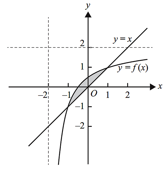
- Find the area of the shaded region. (1 mark)
--- 5 WORK AREA LINES (style=lined) ---
- Part of the graphs of `f` and `f^(-1)` are shown in the diagram below.
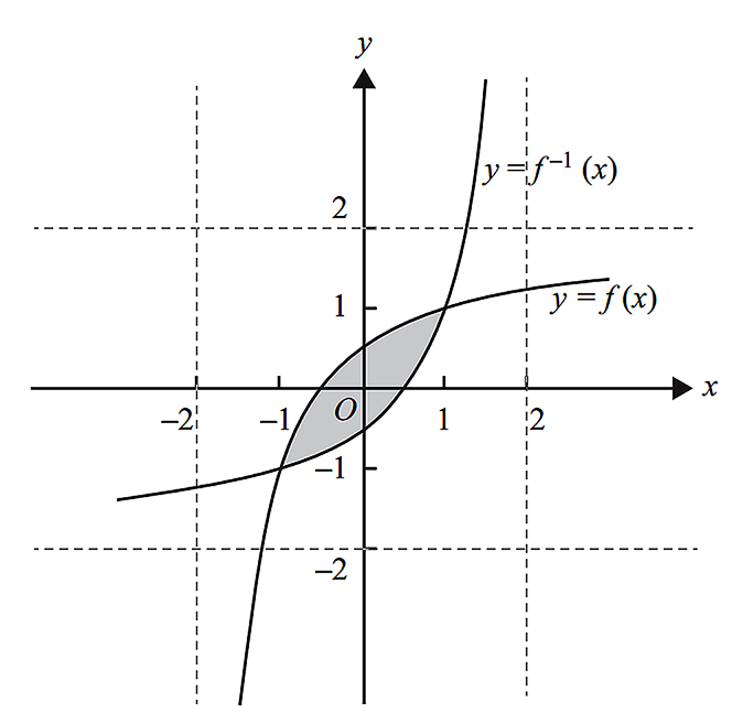
- Find the area of the shaded region. (1 mark)
--- 5 WORK AREA LINES (style=lined) ---
- Find the rule and domain of `f^(-1)`, the inverse function of `f`. (2 marks)


- Part of the graph of `f` is shown in the diagram below.
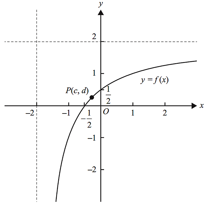
The point `P(c, d)` is on the graph of `f`.
Find the exact values of `c` and `d` such that the distance of this point to the origin is a minimum, and find this minimum distance. (3 marks)
--- 6 WORK AREA LINES (style=lined) ---

Let `g: (−k, oo) -> R, g(x) = (kx + 1)/(x + k)`, where `k > 1`.
- Show that `x_1 < x_2` implies that `g(x_1) < g(x_2),` where `x_1 in (−k, oo) and x_2 in (−k, oo)`. (2 marks)
--- 7 WORK AREA LINES (style=lined) ---
- Let `X` be the point of intersection of the graphs of `y = g (x) and y = −x`.
- Find the coordinates of `X` in terms of `k`. (2 marks)
--- 7 WORK AREA LINES (style=lined) ---
- Find the value of `k` for which the coordinates of `X` are `(-1/2, 1/2)`. (2 marks)
--- 5 WORK AREA LINES (style=lined) ---
- Let `Ztext{(− 1, − 1)}, Y(1, 1)` and `X` be the vertices of the triangle `XYZ`. Let `s(k)` be the square of the area of triangle `XYZ`.
Find the values of `k` such that `s(k) >= 1`. (2 marks)
--- 5 WORK AREA LINES (style=lined) ---
- Find the coordinates of `X` in terms of `k`. (2 marks)
- The graph of `g` and the line `y = x` enclose a region of the plane. The region is shown shaded in the diagram below.
Let `A(k)` be the rule of the function `A` that gives the area of this enclosed region. The domain of `A` is `(1, oo)`.
- Give the rule for `A(k)`. (2 marks)
--- 4 WORK AREA LINES (style=lined) ---
- Show that `0 < A(k) < 2` for all `k > 1`. (2 marks)
--- 6 WORK AREA LINES (style=lined) ---
- Give the rule for `A(k)`. (2 marks)


Show Worked Solution
a. `text(Solution 1)`
| `(2x + 1)/(x + 2)` | `= 2-3/(x + 2)` |
| `= 2 + {(-3)}/(x + 2) qquad [text(CAS: prop Frac) ((2x + 1)/(x + 2))]` |
`text(Solution 2)`
| `(2x + 1)/(x + 2)` | `=(2(x+2)-3)/(x+2)` |
| `=2+ (-3)/(x+2)` |
b.i. `text(Let)\ \ y = f(x)`
`text(For Inverse: swap)\ \ x ↔ y`
| `x` | `=2-3/(y + 2)` |
| `(x-2)(y+2)` | `=-3` |
| `y` | `=(-3)/(x-2)-2` |
`text(Range of)\ f(x):\ \ y in R text(\){2}`
`:. f^(-1) (x) = (-3)/(x-2)-2, \ x in R text(\){2}`
b.ii. `text(Find intersection points:)`
| `f(x)` | `= x` |
| `(2x+1)/(x+2)` | `=x` |
| `2x+1` | `=x^2+2x` |
| `:. x` | `= +- 1` |
| `:.\ text(Area)` | `= int_(-1)^1 (f(x)-x)\ dx` |
| `=int_(-1)^1 (2-3/(x + 2)-x)\ dx` | |
| `= 4-3 ln(3)\ text(u²)` |
| b.iii. | `text(Area)` | `= int_(-1)^1 (f(x)-f^(-1) (x)) dx` |
| `=2 xx (4-3 ln(3))\ \ \ text{(twice the area in (b)(ii))}` | ||
| `= 8-6 log_e (3)\ text(u²)` |
♦♦♦ Mean mark part (c) 25%.
| c. |  |
|
| `text(Let)\ \ z` | `= OP, qquad P(c, -3/(c + 2) + 2)` | |
| `z` | `= sqrt (c^2 + (2-3/(c + 2))^2), \ c > -2` | |
`text(Stationary point when:)`
`(dz)/(dc) = 0, c > -2`
`:.\ c = sqrt 3-2 overset and (->) d = 2-sqrt 3`
`:. text(Minimum distance) = (2 sqrt 2-sqrt 6)`
d. `text(Given:)\ \ -k < x_1 < x_2`
♦♦♦ Mean mark part (d) 8%.
`text(Must prove:)\ \ g(x_2)-g(x_1) > 0`
`text(LHS:)`
`g(x_2)-g(x_1)`
`= (kx_2 +1)/(x_2+k)-(kx_1 +1)/(x_1+k)`
`=((kx_2 +1)(x_1+k)-(kx_1 +1)(x_2+k))/((x_2+k)(x_1+k))`
`=(k^2(x_2-x_1)-(x_2-x_1))/((x_2+k)(x_1+k))`
`=((k^2-1)(x_2-x_1))/((x_2+k)(x_1+k))`
`x_2-x_1 >0,\ and \ k^2-1>0`
`text(S)text(ince)\ \ x_2>x_1> -k,`
`=> -x_2<-x_1<k`
`=>k+x_1 >0, \ and \ k+x_2>0`
`:.g(x_2)-g(x_1) >0`
`:. g(x_2) > g(x_1)`
♦♦ Mean mark part (e)(i) 32%.
| e.i. | `g(x)` | `= -x` |
| `(kx +1)/(x+k)` | `=-x` | |
| `kx+1` | `=-x^2-xk` | |
| `x^2+2k+1` | `=0` | |
| `:. x` | `=(-2k +- sqrt(4k^2-4))/2` | |
| `= sqrt (k^2-1)-k\ \ text(for)\ \ x > -k` |
`:. X (-k + sqrt(k^2-1),\ \ k-sqrt(k^2-1))`
e.ii. `text(Equate)\ \ x text(-coordinates:)`
♦ Mean mark part (e)(ii) 44%.
| `-k + sqrt(k^2-1)` | `= -1/2` |
| `sqrt(k^2-1)` | `=k-1/2` |
| `k^2-1` | `=k^2-k+1/4` |
| `:. k` | `= 5/4` |
| e.iii. | `s(k)` | `= (1/2 xx YZ xx XO)^2` |
| `= 1/4 xx (YZ)^2 xx (XO)^2` |
`ZO = sqrt(1^2+1^2) = sqrt2`
♦♦♦ Mean mark (e)(iii) 6%.
`YZ=2 xx ZO = 2sqrt2`
`(YZ)^2 = 8`
| `(XO)^2` | `=(-k + sqrt(k^2-1))^2-(k-sqrt (k^2-1))^2` |
| `=2(-k + sqrt(k^2-1))^2` | |
`text(Solve)\ \ s(k) >= 1\ \ text(for)\ \ k >= 1,`
| `1/4 xx 8 xx 2(-k + sqrt(k^2-1))^2` | `>=1` |
| `(-k + sqrt(k^2-1))^2` | `>=1/4` |
| `k-sqrt(k^2-1)` | `>=1/2` |
| `k-1/2` | `>= sqrt(k^2-1)` |
| `k^2-k+1/4` | `>=k^2-1` |
| `:.k` | `<= 5/4` |
`:. 1<k<= 5/4`
♦♦ Mean mark (f)(i) 28%.
| f.i. | `A(k)` | `= int_(-1)^1 (g(x)-x)\ dx,\ \ k > 1` |
| `= int_(-1)^1 ((kx+1)/(x+k) -x)\ dx` | ||
| `= int_(-1)^1 (k+ (1-k^2)/(x+k) -x)` | ||
| `=[kx + (1-k^2) log_e(x+k)-x^2/2]_(-1)^1` | ||
| `=(k+(1-k^2)log_e(1+k)-1/2)-(-k+(1-k^2)log_e(k-1)-1/2)` | ||
| `=2k+(1-k^2)log_e ((1+k)/(k-1))` | ||
| `= (k^2-1) log_e ((k-1)/(k + 1)) + 2k` |
♦♦♦ Mean mark part (f)(ii) 4%.
| f.ii. |  |
|
| `0` | `< A(k) < text(Area of)\ Delta ABC` | |
| `0` | `< A(k) < 1/2 xx AC xx BO` | |
| `0` | `< A(k) < 1/2 sqrt(2^2 + 2^2) xx (sqrt(1^2 + 1^2))` | |
| `0` | `< A(k) < 1/2 xx 2 sqrt 2 xx sqrt 2` | |
| `:. 0` | `< A(k) < 2` | |
MATRICES, FUR2 2016 VCAA 3
A travel company is studying the choice between air (`A`), land (`L`), sea (`S`) or no (`N`) travel by some of its customers each year.
Matrix `T`, shown below, contains the percentages of customers who are expected to change their choice of travel from year to year.
`{:(qquadqquadqquadqquadqquadquadtext(this year)),(qquadqquadqquadquadAqquadqquadLqquadqquadSqquadquadN),(T = [(0.65,0.25,0.25,0.50),(0.15,0.60,0.20,0.15),(0.05,0.10,0.25,0.20),(0.15,0.05,0.30,0.15)]{:(A),(L),(S),(N):}text(next year)):}`
Let `S_n` be the matrix that shows the number of customers who choose each type of travel `n` years after 2014.
Matrix `S_0` below shows the number of customers who chose each type of travel in 2014.
`S_0 = [(520),(320),(80),(80)]{:(A),(L),(S),(N):}`
Matrix `S_1` below shows the number of customers who chose each type of travel in 2015.
`S_1 = TS_0 = [(478),(d),(e),(f)]{:(A),(L),(S),(N):}`
- Find the values missing from matrix `S_1 (d, e, f )`. (1 mark)
--- 2 WORK AREA LINES (style=lined) ---
- Write a calculation that shows that 478 customers were expected to choose air travel in 2015. (1 mark)
--- 2 WORK AREA LINES (style=lined) ---
- Consider the customers who chose sea travel in 2014.
- How many of these customers were expected to choose sea travel in 2015? (1 mark)
--- 3 WORK AREA LINES (style=lined) ---
- Consider the customers who were expected to choose air travel in 2015.
- What percentage of these customers had also chosen air travel in 2014?
- Round your answer to the nearest whole number. (1 mark)
--- 4 WORK AREA LINES (style=lined) ---
In 2016, the number of customers studied was increased to 1360.
Matrix `R_2016`, shown below, contains the number of these customers who chose each type of travel in 2016.
`R_2016 = [(646),(465),(164),(85)]{:(A),(L),(S),(N):}`
- The company intends to increase the number of customers in the study in 2017 and in 2018.
- The matrix that contains the number of customers who are expected to choose each type of travel in 2017 (`R_2017`) and 2018 (`R_2018`) can be determined using the matrix equations shown below.
`R_2017 = TR_2016 + BqquadqquadqquadR_2018 = TR_2017 + B`
`{:(qquadqquadqquadqquadqquadquadtext(this year)),(qquadqquadqquadquadAqquadqquadLqquadqquadSqquadquadN),(T = [(0.65,0.25,0.25,0.50),(0.15,0.60,0.20,0.15),(0.05,0.10,0.25,0.20),(0.15,0.05,0.30,0.15)]{:(A),(L),(S),(N):}text(next year)):}qquadqquad{:(),(),(B = [(80),(80),(40),(−80)]{:(A),(L),(S),(N):}):}`
-
- The element in the fourth row of matrix `B` is – 80.
- Explain this number in the context of selecting customers for the studies in 2017 and 2018. (1 mark)
--- 2 WORK AREA LINES (style=lined) ---
- Determine the number of customers who are expected to choose sea travel in 2018.
- Round your answer to the nearest whole number. (2 marks)
--- 5 WORK AREA LINES (style=lined) ---
CORE, FUR1 2016 VCAA 6-7 MC
Part 1
The histogram below shows the distribution of the number of billionaires per million people for 53 countries.

Using this histogram, the percentage of these 53 countries with less than two billionaires per million people is closest to
- `text(49%)`
- `text(53%)`
- `text(89%)`
- `text(92%)`
- `text(98%)`
Part 2
The histogram below shows the distribution of the number of billionaires per million people for the same 53 countries as in Part 1, but this time plotted on a `log_10` scale.

Based on this histogram, the number of countries with one or more billionaires per million people is
- `text(1)`
- `text(3)`
- `text(8)`
- `text(9)`
- `text(10)`
MATRICES, FUR2 2013 VCAA 2
10 000 trout eggs, 1000 baby trout and 800 adult trout are placed in a pond to establish a trout population.
In establishing this population
-
- eggs (`E`) may die (`D`) or they may live and eventually become baby trout (`B`)
- baby trout (`B`) may die (`D`) or they may live and eventually become adult trout (`A`)
- adult trout (`A`) may die (`D`) or they may live for a period of time but will eventually die.
From year to year, this situation can be represented by the transition matrix `T`, where
`{:(qquadqquadqquadqquadqquadtext(this year)),((qquadqquadqquadE,quad\ B,quad\ A,\ D)),(T = [(0,0,0,0),(0.4,0,0,0),(0,0.25,0.5,0),(0.6,0.75,0.5,1)]):}{:(),(),(E),(B),(A),(D):}{:(),(),(qquadtext(next year)):}`
- Use the information in the transition matrix `T` to
- determine the number of eggs in this population that die in the first year. (1 mark)
--- 2 WORK AREA LINES (style=lined) ---
- complete the transition diagram below, showing the relevant percentages. (2 marks)
--- 0 WORK AREA LINES (style=lined) ---
- determine the number of eggs in this population that die in the first year. (1 mark)

The initial state matrix for this trout population, `S_0`, can be written as
`S_0 = [(10\ 000),(1000),(800),(0)]{:(E),(B),(A),(D):}`
Let `S_n` represent the state matrix describing the trout population after `n` years.
- Using the rule `S_n = T S_(n-1)`, determine each of the following.
- `S_1` (1 mark)
--- 3 WORK AREA LINES (style=lined) ---
- the number of adult trout predicted to be in the population after four years (1 mark)
--- 3 WORK AREA LINES (style=lined) ---
- `S_1` (1 mark)
- The transition matrix `T` predicts that, in the long term, all of the eggs, baby trout and adult trout will die.
- How many years will it take for all of the adult trout to die (that is, when the number of adult trout in the population is first predicted to be less than one)? (1 mark)
--- 2 WORK AREA LINES (style=lined) ---
- What is the largest number of adult trout that is predicted to be in the pond in any one year? (1 mark)
--- 3 WORK AREA LINES (style=lined) ---
- How many years will it take for all of the adult trout to die (that is, when the number of adult trout in the population is first predicted to be less than one)? (1 mark)
- Determine the number of eggs, baby trout and adult trout that, if added to or removed from the pond at the end of each year, will ensure that the number of eggs, baby trout and adult trout in the population remains constant from year to year. (2 marks)
--- 4 WORK AREA LINES (style=lined) ---
The rule `S_n = T S_(n – 1)` that was used to describe the development of the trout in this pond does not take into account new eggs added to the population when the adult trout begin to breed.
- To take breeding into account, assume that 50% of the adult trout lay 500 eggs each year.
- The matrix describing the population after one year, `S_1`, is now given by the new rule
- `S_1 = T S_0 + 500\ M\ S_0`
- where `T=[(0,0,0,0),(0.40,0,0,0),(0,0.25,0.50,0),(0.60,0.75,0.50,1.0)], M=[(0,0,0.50,0),(0,0,0,0),(0,0,0,0),(0,0,0,0)]\ text(and)\ S_0=[(10\ 000),(1000),(800),(0)]`
- Use this new rule to determine `S_1`. (1 mark)
--- 4 WORK AREA LINES (style=lined) ---
- Use this new rule to determine `S_1`. (1 mark)
- This pattern continues so that the matrix describing the population after `n` years, `S_n`, is given by the rule
- `S_n = T\ S_(n-1) + 500\ M\ S_(n-1)`
- Use this rule to determine the number of eggs in the population after two years (2 marks)
--- 6 WORK AREA LINES (style=lined) ---
- Use this rule to determine the number of eggs in the population after two years (2 marks)
Show Worked Solution
a.i. `text(60% of eggs die in 1st year,)`
`:.\ text(Eggs that die in year 1)`
`= 0.60 xx 10\ 000`
`= 6000`
MARKER’S COMMENT: A 100% cycle drawn at `D` was a common omission. Do not draw loops and edges of 0%!
| a.ii. |
|

| b.i. | `S_1` | `= TS_0` |
| `= [(0,0,0,0),(0.4,0,0,0),(0,0.25,0.5,0),(0.6,0.75,0.5,1)][(10\ 000),(1000),(800),(0)]= [(0),(4000),(650),(7150)]` |
| b.ii. | `S_4` | `= T^4S_0` |
| `= [(0,0,0,0),(0.4,0,0,0),(0,0.25,0.5,0),(0.6,0.75,0.5,1)]^4[(10\ 000),(1000),(800),(0)]= [(0),(0),(331.25),(11\ 468.75)]` |
`:. 331\ text(trout is the predicted population after 4 years.)`
| c.i. | `S_12 = T^12S_0 = [(0),(0),(1.29),(11\ 791)]` |
`S_13 = T^13S_0 = [(0),(0),(0.65),(11\ 799)]`
`:.\ text{It will take 13 years (when the trout population drops below 1).}`
| c.ii. | `S_1 = TS_0 = [(0),(4000),(650),(7150)]` |
`text(After 1 year, 650 adult trout.)`
`text(Similarly,)`
`S_2 = T^2S_0 = [(0),(0),(1325),(10\ 475)]`
`S_3 = T^3S_0 = [(0),(0),(662.5),(11\ 137.5)]`
`S_4 = T^4S_0 = [(0),(0),(331),(11\ 469)]`
`:.\ text(Largest number of adult trout = 1325.)`
| d. | `S_0-S_1 = [(10\ 000),(1000),(800),(0)]-[(0),(4000),(650),(7150)] = [(10\ 000),(−3000),(150),(−7150)]` |
`:.\ text(Add 10 000 eggs, remove 3000 baby trout and add 150 adult)`
`text(trout to keep the population constant.)`
| e.i. | `S_1` | `= TS_0 + 500MS_0` |
| `= [(0),(4000),(650),(7150)] + 500 xx [(0,0,0.5,0),(0,0,0,0),(0,0,0,0),(0,0,0,0)][(10\ 000),(1000),(800),(0)]` | ||
| `= [(0),(4000),(650),(7150)] + 500[(400),(0),(0),(0)]` | ||
| `= [(200\ 000),(4000),(650),(7150)]` |
| e.ii. | `S_2` | `= TS_1 + 500MS_1` |
|
`= [(0,0,0,0),(0.4,0,0,0),(0,0.25,0.5,0),(0.6,0.75,0.5,1)][(200\ 000),(4000),(650),(7150)]` `+ 500 xx [(0,0,0.5,0),(0,0,0,0),(0,0,0,0),(0,0,0,0)][(200\ 000),(4000),(650),(7150)]` |
||
| `= [(162\ 500),(80\ 000),(1325),(130\ 475)]` |
MATRICES, FUR1 2013 VCAA 7 MC
A school has three computer classes, A, B and C. There are 15 students in each class.
Each student is given a mark out of 100 based on their performance in a test.
Matrix `M` below displays the marks obtained by these 45 students, listed by class.
`M = [(56,78,79,43,67,56,80,85,75,89,55,64,95,34,63), (90,45,56,65,76,79,27,45,69,73,70,63,65,34,59), (76,76,89,47,50,66,68,89,88,90,45,67,78,45,87)]{:(A),(B),(C):} quad text (class)`
Two other matrices, `S` and `R`, are defined below.
`S = [(1),(1),(1),(1),(1),(1),(1),(1),(1),(1),(1),(1),(1),(1),(1)] quad text(and) quad R = [(1,1,1)]`
Which one of the following matrix expressions can be used to generate a matrix that displays the mean mark obtained for each class?
A. `1/45M`
B. `1/3R×M`
C. `1/3R×M×S`
D. `1/15M×S`
E. `1/15S×R×M`
Calculus, 2ADV C3 2004 HSC 10b

The diagram shows a triangular piece of land `ABC` with dimensions `AB = c` metres, `AC = b` metres and `BC = a` metres, where `a ≤ b ≤ c`.
The owner of the land wants to build a straight fence to divide the land into two pieces of equal area. Let `S` and `T` be points on `AB` and `AC` respectively so that `ST` divides the land into two pieces of equal area.
Let `AS = x` metres, `AT = y` metres and `ST = z` metres.
- Show that `xy = 1/2 bc`. (1 mark)
--- 2 WORK AREA LINES (style=lined) ---
- Use the cosine rule in triangle `AST` to show that
`z^2 = x^2 + (b^2c^2)/(4x^2) − bc cos A.` (2 marks)
--- 5 WORK AREA LINES (style=lined) ---
- Show that the value of `z^2` in the equation in part (ii) is a minimum when
`x = sqrt((bc)/2)`. (4 marks)
--- 8 WORK AREA LINES (style=lined) ---
- Show that the minimum length of the fence is `sqrt(((P − 2b)(P − 2c))/2)` metres, where `P = a + b + c`.
(You may assume that the value of `x` given in part (iii) is feasible.) (2 marks)
--- 5 WORK AREA LINES (style=lined) ---
Functions, EXT1′ F1 2015 HSC 8 MC
The graph of the function `y = f(x)` is shown.

A second graph is obtained from the function `y = f(x).`

Which equation best represents the second graph?
- `y^2 = |\ f(x)\ |`
- `y^2 = f(x)`
- `y = sqrt (f(x))`
- `y = f(sqrt x)`
Algebra, STD2 A4 2007 HSC 27a
A rectangular playing surface is to be constructed so that the length is 6 metres more than the width.
- Give an example of a length and width that would be possible for this playing surface. (1 mark)
--- 2 WORK AREA LINES (style=lined) ---
- Write an equation for the area (`A`) of the playing surface in terms of its length (`l`). (1 mark)
--- 1 WORK AREA LINES (style=lined) ---
A graph comparing the area of the playing surface to its length is shown.
- Why are lengths of 0 metres to 6 metres impossible? (1 mark)
--- 2 WORK AREA LINES (style=lined) ---
- What would be the dimensions of the playing surface if it had an area of 135 m²? (2 marks)
--- 4 WORK AREA LINES (style=lined) ---
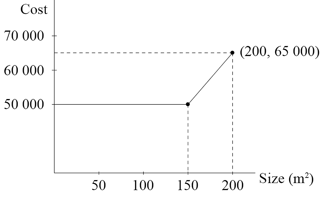
Company `A` constructs playing surfaces.
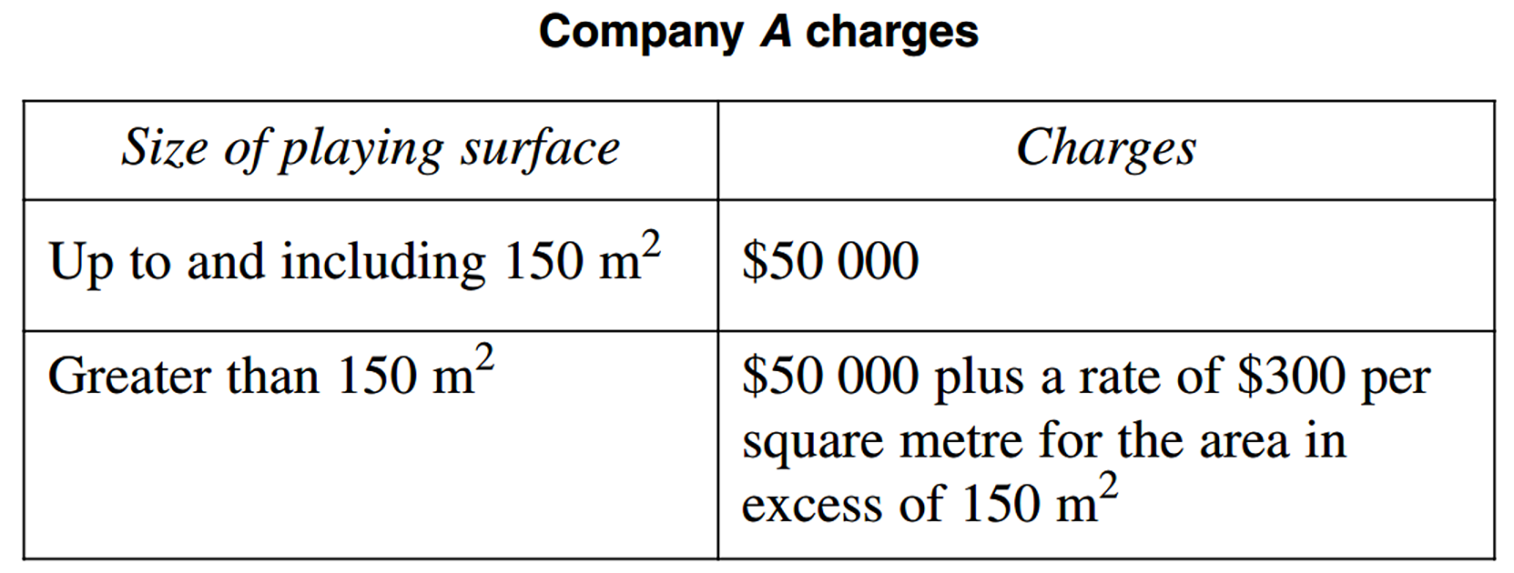
- Draw a graph to represent the cost of using Company `A` to construct all playing surface sizes up to and including 200 m².
Use the horizontal axis to represent the area and the vertical axis to represent the cost. (2 marks)
--- 8 WORK AREA LINES (style=lined) ---
- Company `B` charges a rate of $360 per square metre regardless of size.
- Which company would charge less to construct a playing surface with an area of 135 m²
Justify your answer with suitable calculations. (1 mark)
--- 2 WORK AREA LINES (style=lined) ---


Show Answers Only
- `text(One possibility is a length of 10 m, and a width)`
`text{of 4 m (among many possibilities).}`
- `A = l (l – 6)\ \ text(m²)`
- `text(Given the length must be 6 m more than)`
`text(the width, it follows that the length)`
`text(must be greater than 6 m.)`
- `text(15 m × 9 m)`
-
- `text(Proof)\ \ text{(See worked solutions)}`
Show Worked Solution
i. `text(One possibility is a length of 10 m, and a width)`
`text{of 4 m (among many possibilities).}`
ii. `text(Length) = l\ text(m)`
`text(Width) = (l – 6)\ text(m)`
| `:.\ A` | `= l (l – 6)` |
iii. `text(Given the length must be 6m more than the width,)`
`text(it follows that the length must be greater than 6 m)`
`text(so that the width is positive.)`
iv. `text(From the graph, an area of 135 m² corresponds to)`
`text(a length of 15 m.)`
`:.\ text(The dimensions would be 15 m × 9 m.)`
| v. |  |
vi. `text(Company)\ A\ text(cost) = $50\ 000`
| `text(Company)\ B\ text(cost)` | `= 135 xx 360` |
| `= $48\ 600` |
`:.\ text(Company)\ B\ text(would charge $1400 less)`
`text(than Company)\ A.`
CORE, FUR1 2014 VCAA 6 MC
The dot plot below shows the distribution of the time, in minutes, that 50 people spent waiting to get help from a call centre.

Which one of the following boxplots best represents the data?


Statistics, STD2 S5 2008 HSC 28a
The following graph indicates `z`-scores of ‘height-for-age’ for girls aged 5 – 19 years.

- What is the `z`-score for a six year old girl of height 120 cm? (1 mark)
--- 2 WORK AREA LINES (style=lined) ---
- Rachel is 10 ½ years of age.
(1) If 2.5% of girls of the same age are taller than Rachel, how tall is she? (1 mark)
--- 1 WORK AREA LINES (style=lined) ---
(2) Rachel does not grow any taller. At age 15 ½, what percentage of girls of the same age will be taller than Rachel? (2 marks)
--- 4 WORK AREA LINES (style=lined) ---
- What is the average height of an 18 year old girl? (1 mark)
--- 1 WORK AREA LINES (style=lined) ---
For adults (18 years and older), the Body Mass Index is given by
`B = m/h^2` where `m = text(mass)` in kilograms and `h = text(height)` in metres.
The medically accepted healthy range for `B` is `21 <= B <= 25`.
- What is the minimum weight for an 18 year old girl of average height to be considered healthy? (2 marks)
--- 4 WORK AREA LINES (style=lined) ---
- The average height, `C`, in centimetres, of a girl between the ages of 6 years and 11 years can be represented by a line with equation
`C = 6A + 79` where `A` is the age in years.
(1) For this line, the gradient is 6. What does this indicate about the heights of girls aged 6 to 11? (1 mark)
--- 2 WORK AREA LINES (style=lined) ---
(2) Give ONE reason why this equation is not suitable for predicting heights of girls older than 12. (1 mark)
--- 2 WORK AREA LINES (style=lined) ---
FS Resources, 2UG 2014 HSC 28d
An aerial diagram of a swimming pool is shown.

The swimming pool is a standard length of 50 metres but is not in the shape of a rectangle.
(i) Given `AB=8\ text(cm)`, determine the scale of the diagram such that
1 cm = `x` m (1 mark)
(ii) If the length of a carpark next to the pool measured 5 cm (not shown), how long would it be in real life? (1 mark)
(iii) In the diagram of the swimming pool, the five widths are measured to be:
`CD = 21.88\ text(m)`
`EF = 25.63\ text(m)`
`GH = 31.88\ text(m)`
`IJ = 36.25\ text(m)`
`KL = 21.88\ text(m)`
The average depth of the pool is 1.2 m
Calculate the approximate volume of the swimming pool, in cubic metres. In your calculations, use TWO applications of Simpson’s Rule. (3 marks)
Show Worked Solution
| (i) | `\ \ \ \ 8\ text(cm)` | `=50\ text(m)` |
| `1\ text(cm)` | `=50/8` | |
| `=6.25\ text(m)` |
`:.x=6.25\ text(m)`
(ii) `text{Using scale from (i)}`
| `5\ text(cm)` | `=5 xx 6.25` |
| `=31.25\ text(m)` |
`:.\ text(The carpark would be 31.25 m long)`
| (iii) |  |
`h = 50/4 = 12.5\ text(m)`
♦ Mean mark 50%. Be careful not to give away easy marks!
| `A` | `~~ h/3 [y_0 + 4(y_1) + y_2]\ \ text(… applied twice)` |
| `~~ 12.5/3 [21.88 + 4(25.63) + 31.88]` | |
| `+ 12.5/3 [31.88 + 4(36.25) + 21.88]` | |
| `~~ 12.5/3 [156.28] + 12.5/3 [198.76]` | |
| `~~ 1,479.33\ text(m²)` |
| `V` | `= Ah` |
| `~~ 1479.33 xx 1.2` | |
| `~~ 1775.2` | |
| `~~ 1775\ text(m³)` |
Inverse Functions, EXT1 2013 HSC 2 MC
The diagram shows the graph `y = f(x)`.

Which diagram shows the graph `y = f^(-1) (x)`?


Show Worked Solution

`f^(-1) (x)\ text(is the reflection of)\ \ f(x)\ \ text(in the line)\ y = x`
`=> D`
Measurement, STD2 M7 2011 HSC 24a
Part of the floor plan of a house is shown. The plan is drawn to scale.

- What is the width of the stairwell, in millimetres? (1 mark)
--- 2 WORK AREA LINES (style=lined) ---
- What are the internal dimensions of the bathroom, in millimetres? (1 mark)
--- 2 WORK AREA LINES (style=lined) ---
- What is the length `AB`, the internal length of the rumpus room, in millimetres? (1 mark)
--- 2 WORK AREA LINES (style=lined) ---
Measurement, STD2 M1 2010 HSC 28b
Moivre’s manufacturing company produces cans of Magic Beans. The can has a diameter of 10 cm and a height of 10 cm.

- Cans are packed in boxes that are rectangular prisms with dimensions 30 cm × 40 cm × 60 cm.
What is the maximum number of cans that can be packed into one of these boxes? (1 mark)
--- 2 WORK AREA LINES (style=lined) ---
- The shaded label on the can shown wraps all the way around the can with no overlap. What area of paper is needed to make the labels for all the cans in this box when the box is full? (2 marks)
--- 4 WORK AREA LINES (style=lined) ---
- The company is considering producing larger cans. Monica says if you double the diameter of the can this will double the volume.
Is Monica correct? Justify your answer with suitable calculations. (2 marks)
--- 5 WORK AREA LINES (style=lined) ---
The company wants to produce a can with a volume of 1570 cm³, using the least amount of metal. Monica is given the job of determining the dimensions of the can to be produced. She considers the following graphs.
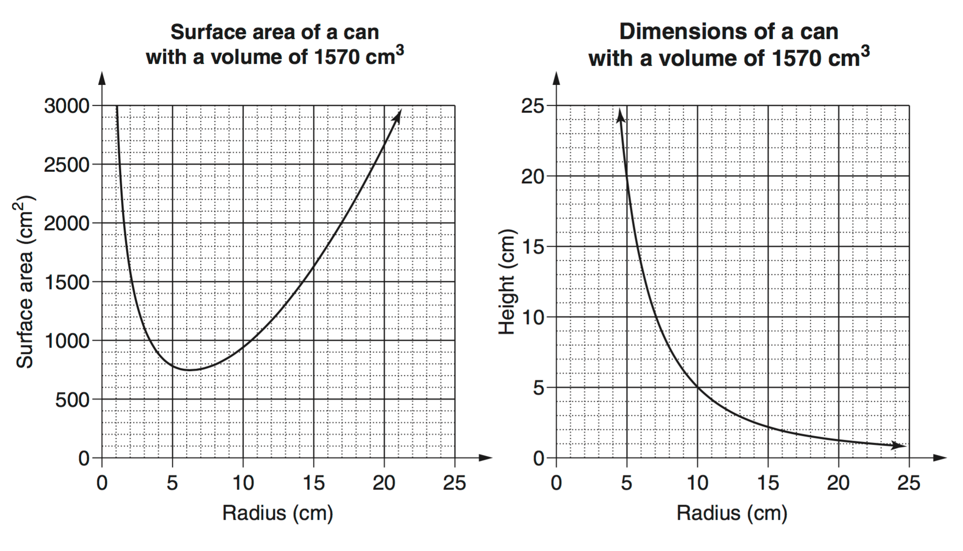
- What radius and height should Monica recommend that the company use to minimise the amount of metal required to produce these cans? Justify your choice of dimensions with reference to the graphs and/or suitable calculations. (2 marks)
--- 5 WORK AREA LINES (style=lined) ---

Show Worked Solution
♦♦ Mean mark 27%
| a. | `text(Maximum # Cans)` | `= 4 xx 3 xx 6` |
| `= 72\ text(cans)` |
♦ Mean mark 38%
MARKER’S COMMENT: Many students didn’t account for the clearance of 0.5 cm at the top and bottom of each can.
MARKER’S COMMENT: Many students didn’t account for the clearance of 0.5 cm at the top and bottom of each can.
| b. | `text(Label Area)\ text{(1 can)}` | `= 2 pi rh` |
| `= 2 xx pi xx 5 xx 9` | ||
| `= 90 pi` | ||
| `= 282.7433…\ text(cm²)` |
`:.\ text(Label Area)\ text{(72 cans)}`
`= 72 xx 282.7433…`
`= 20\ 357.52…`
`= 20\ 358\ text(cm²)` `text{(nearest cm²)}`
♦ Mean mark 44%
MARKER’S COMMENT: Many students performed calculations in this part without concluding if Monica is correct or not. Read the question carefully.
MARKER’S COMMENT: Many students performed calculations in this part without concluding if Monica is correct or not. Read the question carefully.
| c. | `text(Original volume)` | `= pi r^2 h` |
| `= pi xx 5^2 xx 10` | ||
| `= 785.398…\ text(cm³)` |
| `text(If the diameter doubles, radius) = 10\ text(cm)` |
| `text(New volume)` | `= pi xx 10^2 xx 10` |
| `= 3141.592…\ text(cm³)` |
| `:.\ text(Monica is incorrect because the volume)` |
| `text(doesn’t double. It increases by a factor of 4.)` |
♦♦ Mean mark 26%
| d. |  |
| `text(Minimum metal used when surface area is a minimum.)` |
| `text(From graph, minimum surface area when)\ r = 6.3\ text(cm)` |
| `text(When)\ r = 6.3\ text(cm,)\ h = 12.6\ text(cm)\ \ \ text{(from graph)}` |
| `:.\ text(She should recommend radius 6.3 cm and height 12.6 cm)` |
Financial Maths, STD2 F4 2010 HSC 28a
The table shows monthly home loan repayments with interest rate changes from February to October 2009.

- What is the change in monthly repayments on a $250 000 loan from February 2009 to April 2009? (1 mark)
--- 3 WORK AREA LINES (style=lined) ---
- Xiang wants to borrow $307 000 to buy a house.
Xiang’s bank approves loans for customers if their loan repayments are no more than 30% of their monthly gross salary.
Xiang’s monthly gross salary is $6500.
If she had applied for the loan in October 2009, would her bank have approved her loan?
Justify your answer with suitable calculations. (3 marks)
--- 6 WORK AREA LINES (style=lined) ---
- Jack took out a loan at the same time and for the same amount as Xiang.
Graphs of their loan balances are shown.
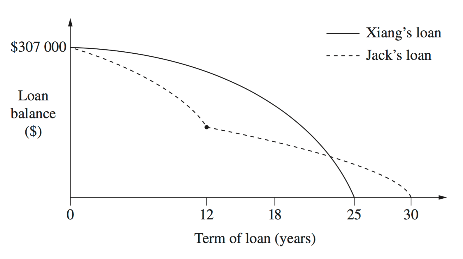
Identify TWO differences between the graphs and provide a possible explanation for each difference, making reference to interest rates and/or loan repayments. (2 marks)
--- 5 WORK AREA LINES (style=lined) ---

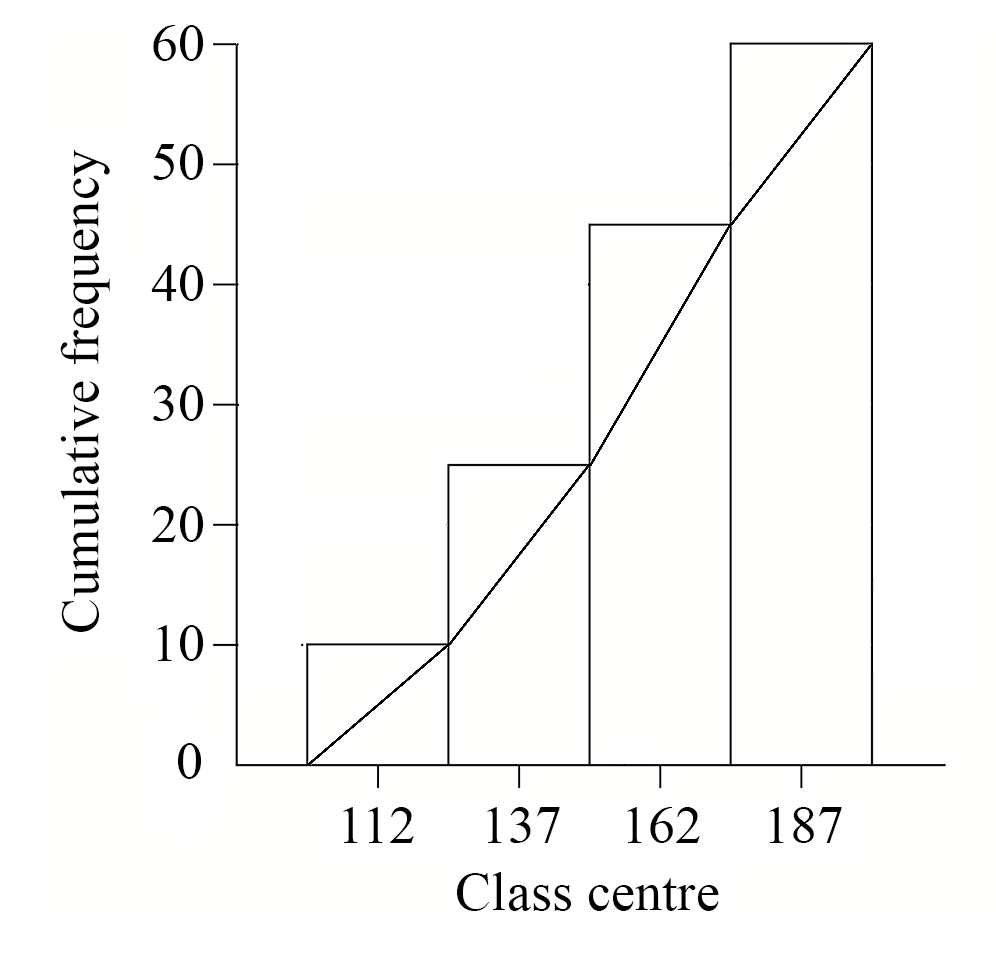
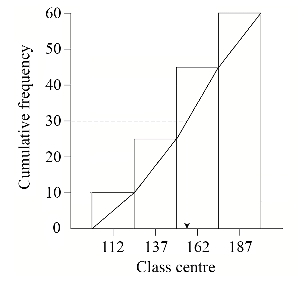
Statistics, STD2 S1 2010 HSC 26b
A new shopping centre has opened near a primary school. A survey is conducted to determine the number of motor vehicles that pass the school each afternoon between 2.30 pm and 4.00 pm.
The results for 60 days have been recorded in the table and are displayed in the cumulative frequency histogram.

- Find the value of Χ in the table. (1 mark)
--- 1 WORK AREA LINES (style=lined) ---
- On the cumulative frequency histogram above, draw a cumulative frequency polygon (ogive) for this data. (1 mark)
- Use your graph to determine the median. Show, by drawing lines on your graph, how you arrived at your answer. (1 mark)
- Prior to the opening of the new shopping centre, the median number of motor vehicles passing the school between 2.30 pm and 4.00 pm was 57 vehicles per day.
What problem could arise from the change in the median number of motor vehicles passing the school before and after the opening of the new shopping centre?
Briefly recommend a solution to this problem. (2 marks)
--- 5 WORK AREA LINES (style=lined) ---
Show Answers Only
- `15`
-
-
- `text(Problems)`
- `text(- increased traffic delays)`
- `text(- increased danger to students leaving school)`
-
`text(Solutions)`
- `text(- signpost alternative routes around school)`
- `text(- decrease the speed limit in the area)`
Show Worked Solution
| a. | `X` | `= 25\ -10` |
| `= 15` |
♦♦♦ Mean mark 18%
MARKER’S COMMENT: The ogive was poorly drawn with many students incorrectly joining the middle of each column rather than from corner to corner.
MARKER’S COMMENT: The ogive was poorly drawn with many students incorrectly joining the middle of each column rather than from corner to corner.
| b. |  |
♦♦ Mean mark 25%
MARKER’S COMMENT: Many students did not “show by drawing lines on the graph” as the question asked.
MARKER’S COMMENT: Many students did not “show by drawing lines on the graph” as the question asked.
c. `text(Median)\ ~~155`

♦ Mean mark 47%
MARKER’S COMMENT: Short answers were often the best. Be concise when you can.
MARKER’S COMMENT: Short answers were often the best. Be concise when you can.
| d. | `text(Problems)` |
| `text(- increased traffic delays)` | |
| `text(- increased danger to students leaving school)` | |
| `text(Solutions)` | |
| `text(- signpost alternative routes around school)` | |
| `text(- decrease the speed limit in the area)` |
Algebra, STD2 A4 2013 HSC 30a
Wind turbines, such as those shown, are used to generate power.

In theory, the power that could be generated by a wind turbine is modelled using the equation
`T = 20\ 000w^3`
| where | `T` is the theoretical power generated, in watts |
| `w` is the speed of the wind, in metres per second. |
- Using this equation, what is the theoretical power generated by a wind turbine if the wind speed is 7.3 m/s ? (1 mark)
--- 1 WORK AREA LINES (style=lined) ---
In practice, the actual power generated by a wind turbine is only 40% of the theoretical power.
- If `A` is the actual power generated, in watts, write an equation for `A` in terms of `w`. (1 mark)
--- 2 WORK AREA LINES (style=lined) ---
The graph shows both the theoretical power generated and the actual power generated by a particular wind turbine.
- Using the graph, or otherwise, find the difference between the theoretical power and the actual power generated when the wind speed is 9 m/s. (1 mark)
--- 1 WORK AREA LINES (style=lined) ---
A particular farm requires at least 4.4 million watts of actual power in order to be self-sufficient.
- What is the minimum wind speed required for the farm to be self-sufficient? (1 mark)
--- 1 WORK AREA LINES (style=lined) ---
A more accurate formula to calculate the power (`P`) generated by a wind turbine is
`P = 0.61 xx pi xx r^2 × w^3`
| where | `r` is the length of each blade, in metres |
| `w` is the speed of the wind, in metres per second. |
Each blade of a particular wind turbine has a length of 43 metres.The turbine operates at a wind speed of 8 m/s.
- Using the formula above, if the wind speed increased by 10%, what would be the percentage increase in the power generated by this wind turbine? (3 marks)
--- 6 WORK AREA LINES (style=lined) ---
Algebra, STD2 A4 2012 HSC 30b
A golf ball is hit from point `A` to point `B`, which is on the ground as shown. Point `A` is 30 metres above the ground and the horizontal distance from point `A` to point `B` is 300 m.

The path of the golf ball is modelled using the equation
`h = 30 + 0.2d-0.001d^2`
where
`h` is the height of the golf ball above the ground in metres, and
`d` is the horizontal distance of the golf ball from point `A` in metres.
The graph of this equation is drawn below.

- What is the maximum height the ball reaches above the ground? (1 mark)
--- 1 WORK AREA LINES (style=lined) ---
- There are two occasions when the golf ball is at a height of 35 metres.
What horizontal distance does the ball travel in the period between these two occasions? (1 mark)
--- 2 WORK AREA LINES (style=lined) ---
- What is the height of the ball above the ground when it still has to travel a horizontal distance of 50 metres to hit the ground at point `B`? (1 mark)
--- 2 WORK AREA LINES (style=lined) ---
- Only part of the graph applies to this model.
Find all values of `d` that are not suitable to use with this model, and explain why these values are not suitable. (2 marks)
--- 4 WORK AREA LINES (style=lined) ---